

208
Air Pollution and Turbulence: Modeling and Applications
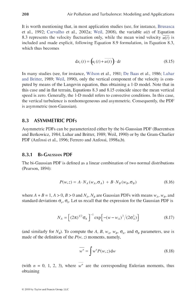
It is worth mentioning that, in most application studies (see, for instance, Brusasca
et al., 1992; Carvalho et al., 2002a; Weil, 2008), the variable u(t) of Equation
8.3 represents the velocity fl uctuation only, while the mean wind velocity ( )
u t is
included and made explicit, following Equation 8.9 formulation, in Equation 8.3,
which thus becomes
(
)
d ( )
( ) ( ) d
i
i
x t
u t u t
t
=
+
⋅
(8.15)
In many studies (see, for instance, Wilson et al., 1981; De Baas et al., 1986; Luhar
and Britter, 1989; Weil, 1990), only the vertical component of the velocity is computed by means of the Langevin equation, thus obtaining a 1-D model. Note that in
this case and in fl at terrain, Equations 8.3 and 8.15 coincide since the mean vertical
speed is zero. Generally, the 1-D model refers to convective conditions. In this case,
the vertical turbulence is nonhomogeneous and asymmetric. Consequently, the PDF
is asymmetric (non-Gaussian).
8.3 ASYMMETRIC PDFS
Asymmetric PDFs can be parameterized either by the bi-Gaussian PDF (Baerentsen
and Berkowicz, 1984; Luhar and Britter, 1989; Weil, 1990) or by the Gram-Charlier
PDF (Anfossi et al., 1996; Ferrero and Anfossi, 1998a,b).
8.3.1 BI-GAUSSIAN PDF
The bi-Gaussian PDF is defi ned as a linear combination of two normal distributions
(Pearson, 1894):
( , )
( , )
( , )
A
A
A
B
B
B
P w z
A N w
B N w
= ⋅
σ + ⋅
σ
(8.16)
where A + B = 1, A > 0, B > 0 and N A , N B are Gaussian PDFs with means w A , w B , and
standard deviations σ a , σ b . Let us recall that the expression for the Gaussian PDF is
1
1 2
2
2
(2 )
exp (
) (2 )
A
A
A
A
N
ww
−
⎡
⎤
⎡
⎤
=
π σ
− −
σ
⎣
⎦
⎣
⎦
(8.17)
(and similarly for N B ). To compute the A, B, w A , w B , σ A , and σ B parameters, use is
made of the defi nition of the P(w, z) moments, namely,
=
∫
( , )d
n
n
w
w P w z w
(8.18)
(with n = 0, 1, 2, 3), where
n
w are the corresponding Eulerian moments, thus
obtaining
© 2010 by Taylor and Francis Group, LLC
Air Pollution and Turbulence: Modeling and Applications
It is worth mentioning that, in most application studies (see, for instance, Brusasca
et al., 1992; Carvalho et al., 2002a; Weil, 2008), the variable u(t) of Equation
8.3 represents the velocity fl uctuation only, while the mean wind velocity ( )
u t is
included and made explicit, following Equation 8.9 formulation, in Equation 8.3,
which thus becomes
(
)
d ( )
( ) ( ) d
i
i
x t
u t u t
t
=
+
⋅
(8.15)
In many studies (see, for instance, Wilson et al., 1981; De Baas et al., 1986; Luhar
and Britter, 1989; Weil, 1990), only the vertical component of the velocity is computed by means of the Langevin equation, thus obtaining a 1-D model. Note that in
this case and in fl at terrain, Equations 8.3 and 8.15 coincide since the mean vertical
speed is zero. Generally, the 1-D model refers to convective conditions. In this case,
the vertical turbulence is nonhomogeneous and asymmetric. Consequently, the PDF
is asymmetric (non-Gaussian).
8.3 ASYMMETRIC PDFS
Asymmetric PDFs can be parameterized either by the bi-Gaussian PDF (Baerentsen
and Berkowicz, 1984; Luhar and Britter, 1989; Weil, 1990) or by the Gram-Charlier
PDF (Anfossi et al., 1996; Ferrero and Anfossi, 1998a,b).
8.3.1 BI-GAUSSIAN PDF
The bi-Gaussian PDF is defi ned as a linear combination of two normal distributions
(Pearson, 1894):
( , )
( , )
( , )
A
A
A
B
B
B
P w z
A N w
B N w
= ⋅
σ + ⋅
σ
(8.16)
where A + B = 1, A > 0, B > 0 and N A , N B are Gaussian PDFs with means w A , w B , and
standard deviations σ a , σ b . Let us recall that the expression for the Gaussian PDF is
1
1 2
2
2
(2 )
exp (
) (2 )
A
A
A
A
N
ww
−
⎡
⎤
⎡
⎤
=
π σ
− −
σ
⎣
⎦
⎣
⎦
(8.17)
(and similarly for N B ). To compute the A, B, w A , w B , σ A , and σ B parameters, use is
made of the defi nition of the P(w, z) moments, namely,
=
∫
( , )d
n
n
w
w P w z w
(8.18)
(with n = 0, 1, 2, 3), where
n
w are the corresponding Eulerian moments, thus
obtaining
© 2010 by Taylor and Francis Group, LLC