

An Outline of Lagrangian Stochastic Dispersion Models
207
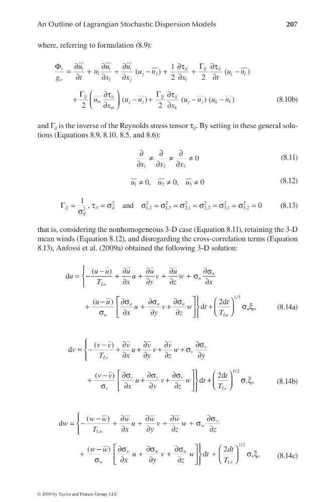
where, referring to formulation (8.9):
1
(
)
(
)
2
2
(
)
(
)(
)
2
2
i
i
i
lj
i
i l
i l
l
j
j
j
j
a
l
j
l
lj
lj
il
il
m
j
j
k
j
j
k
m
k
u
u
u
u
u
u
u
u
g
t
x
x
x
t
u
u
u
u
u
u
u
x
x
Γ
Φ
∂
∂
∂
∂τ
∂τ
=
+
+
−
+
+
−
∂
∂
∂
∂
∂
Γ
Γ
⎛
⎞
∂τ
∂τ
+
− +
−
−
⎜
⎟
⎝
⎠
∂
∂
(8.10b)
and Γ il is the inverse of the Reynolds stress tensor τ il . By setting in these general solutions (Equations 8.9, 8.10, 8.5, and 8.6):
1
2
3
0
x
x
x
∂
∂
∂
≠
≠
≠
∂
∂
∂
(8.11)
≠
≠
≠
1
2
3
0,
0,
0
u
u
u
(8.12)
2
2
2
2
2
2
2
1 , 2
1 , 3
2 , 1
2 , 3
3 , 1
3 , 2
2
1 ,
and
0
lj
il
il
lj
Γ =
τ = σ
σ = σ = σ = σ = σ = σ =
σ
(8.13)
that is, considering the nonhomogeneous 3-D case (Equation 8.11), retaining the 3-D
mean winds (Equation 8.12), and disregarding the cross-correlation terms (Equation
8.13), Anfossi et al. (2009a) obtained the following 3-D solution:
⎧
−
∂
∂
∂
∂
⎪
σ
= −
+
+
+
+ σ
⎨
∂
∂
∂
∂
⎪ ⎩
⎫
⎡
⎤
⎛
⎞
−
∂σ
∂σ
∂σ
⎪
+
+
+
+
σ ξ
⎬
⎢
⎥
⎜
⎟
⎝
⎠
σ
∂
∂
∂
⎪
⎣
⎦ ⎭
1/2
(
)
d
(
)
2d
d
u
u
Lu
u
u
u
u u
u
L u
u u
u
u
u
u
u
v
w
T
x
y
z
x
u u
t
u
v
w
t
x
y
z
T
(8.14a)
⎧
−
∂
∂
∂
∂σ
⎪
= −
+
+
+
+ σ
⎨
∂
∂
∂
∂
⎪ ⎩
⎫
⎡
⎤
⎛
⎞
−
∂σ
∂σ
∂σ
⎪
+
+
+
+
σξ
⎬
⎢
⎥
⎜
⎟
⎝
⎠
σ
∂
∂
∂
⎪
⎣
⎦ ⎭
1/2
(
)
d
(
)
2d
d
v
v
Lv
v
v
v
v v
v
L v
v v
v
v
v
v
u
v
w
T
x
y
z
y
v
t
v
u
v
w
t
x
y
z
T
(8.14b)
⎧
−
∂
∂
∂
∂σ
⎪
= −
+
+
+
+ σ
⎨
∂
∂
∂
∂
⎪ ⎩
⎫
⎡
⎤
⎛
⎞
−
∂σ
∂σ
∂σ
⎪
+
+
+
+
σ ξ
⎬
⎢
⎥
⎜
⎟
⎝
⎠
σ
∂
∂
∂
⎪
⎣
⎦ ⎭
L
1/2
L
(
)
d
(
)
2
d
w
w
w
w
w
w
v v
w
v
w w
w
w
w
w
u
v
w
T
x
y
z
z
w
d t
w
u
v
w
t
x
y
z
T
(8.14c)
© 2010 by Taylor and Francis Group, LLC
207
where, referring to formulation (8.9):
1
(
)
(
)
2
2
(
)
(
)(
)
2
2
i
i
i
lj
i
i l
i l
l
j
j
j
j
a
l
j
l
lj
lj
il
il
m
j
j
k
j
j
k
m
k
u
u
u
u
u
u
u
u
g
t
x
x
x
t
u
u
u
u
u
u
u
x
x
Γ
Φ
∂
∂
∂
∂τ
∂τ
=
+
+
−
+
+
−
∂
∂
∂
∂
∂
Γ
Γ
⎛
⎞
∂τ
∂τ
+
− +
−
−
⎜
⎟
⎝
⎠
∂
∂
(8.10b)
and Γ il is the inverse of the Reynolds stress tensor τ il . By setting in these general solutions (Equations 8.9, 8.10, 8.5, and 8.6):
1
2
3
0
x
x
x
∂
∂
∂
≠
≠
≠
∂
∂
∂
(8.11)
≠
≠
≠
1
2
3
0,
0,
0
u
u
u
(8.12)
2
2
2
2
2
2
2
1 , 2
1 , 3
2 , 1
2 , 3
3 , 1
3 , 2
2
1 ,
and
0
lj
il
il
lj
Γ =
τ = σ
σ = σ = σ = σ = σ = σ =
σ
(8.13)
that is, considering the nonhomogeneous 3-D case (Equation 8.11), retaining the 3-D
mean winds (Equation 8.12), and disregarding the cross-correlation terms (Equation
8.13), Anfossi et al. (2009a) obtained the following 3-D solution:
⎧
−
∂
∂
∂
∂
⎪
σ
= −
+
+
+
+ σ
⎨
∂
∂
∂
∂
⎪ ⎩
⎫
⎡
⎤
⎛
⎞
−
∂σ
∂σ
∂σ
⎪
+
+
+
+
σ ξ
⎬
⎢
⎥
⎜
⎟
⎝
⎠
σ
∂
∂
∂
⎪
⎣
⎦ ⎭
1/2
(
)
d
(
)
2d
d
u
u
Lu
u
u
u
u u
u
L u
u u
u
u
u
u
u
v
w
T
x
y
z
x
u u
t
u
v
w
t
x
y
z
T
(8.14a)
⎧
−
∂
∂
∂
∂σ
⎪
= −
+
+
+
+ σ
⎨
∂
∂
∂
∂
⎪ ⎩
⎫
⎡
⎤
⎛
⎞
−
∂σ
∂σ
∂σ
⎪
+
+
+
+
σξ
⎬
⎢
⎥
⎜
⎟
⎝
⎠
σ
∂
∂
∂
⎪
⎣
⎦ ⎭
1/2
(
)
d
(
)
2d
d
v
v
Lv
v
v
v
v v
v
L v
v v
v
v
v
v
u
v
w
T
x
y
z
y
v
t
v
u
v
w
t
x
y
z
T
(8.14b)
⎧
−
∂
∂
∂
∂σ
⎪
= −
+
+
+
+ σ
⎨
∂
∂
∂
∂
⎪ ⎩
⎫
⎡
⎤
⎛
⎞
−
∂σ
∂σ
∂σ
⎪
+
+
+
+
σ ξ
⎬
⎢
⎥
⎜
⎟
⎝
⎠
σ
∂
∂
∂
⎪
⎣
⎦ ⎭
L
1/2
L
(
)
d
(
)
2
d
w
w
w
w
w
w
v v
w
v
w w
w
w
w
w
u
v
w
T
x
y
z
z
w
d t
w
u
v
w
t
x
y
z
T
(8.14c)
© 2010 by Taylor and Francis Group, LLC