

206
Air Pollution and Turbulence: Modeling and Applications
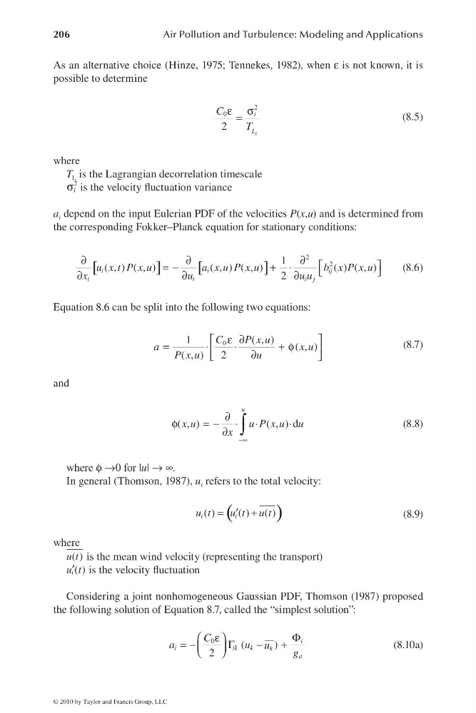
As an alternative choice (Hinze, 1975; Tennekes, 1982), when ε is not known, it is
possible to determine
ε σ
=
2
0
2
i
i
L
C
T
(8.5)
where
T L is the Lagrangian decorrelation timescale
σ
2
i is the velocity fl uctuation variance
a i depend on the input Eulerian PDF of the velocities P(x,u) and is determined from
the corresponding Fokker–Planck equation for stationary conditions:
[
]
[
]
∂
∂
∂ ⎡
⎤
= −
+ ⋅
⎣
⎦
∂
∂
∂
2
2
1
( , ) ( , )
( , ) ( , )
( ) ( , )
2
i
i
i j
i
i
i j
u x t P x u
a x u P x u
b x P x u
x
u
u u
(8.6)
Equation 8.6 can be split into the following two equations:
ε ∂
⎡
⎤
=
⋅
⋅
+φ
⎢
⎥
∂
⎣
⎦
0
1
(,)
( , )
( , )
2
C
P x u
a
x u
P x u
u
(8.7)
and
−∞
∂
φ
= − ⋅
⋅
⋅
∂ ∫
( , )
( , ) d
u
x u
u P x u u
x
(8.8)
where φ →0 for |u| → ∞.
In general (Thomson, 1987), u i refers to the total velocity:
(
)
=
+
′
( )
( ) ( )
i
i
u t
u t u t
(8.9)
where
( )
u t is the mean wind velocity (representing the transport)
′( )
i
u t is the velocity fl uctuation
Considering a joint nonhomogeneous Gaussian PDF, Thomson (1987) proposed
the following solution of Equation 8.7, called the “simplest solution”:
0
(
)
2
i
i
i k
k
k
a
C
a
u u
g
ε
Φ
⎛
⎞
= −
Γ
−
+
⎜
⎟
⎝
⎠
(8.10a)
© 2010 by Taylor and Francis Group, LLC
Air Pollution and Turbulence: Modeling and Applications
As an alternative choice (Hinze, 1975; Tennekes, 1982), when ε is not known, it is
possible to determine
ε σ
=
2
0
2
i
i
L
C
T
(8.5)
where
T L is the Lagrangian decorrelation timescale
σ
2
i is the velocity fl uctuation variance
a i depend on the input Eulerian PDF of the velocities P(x,u) and is determined from
the corresponding Fokker–Planck equation for stationary conditions:
[
]
[
]
∂
∂
∂ ⎡
⎤
= −
+ ⋅
⎣
⎦
∂
∂
∂
2
2
1
( , ) ( , )
( , ) ( , )
( ) ( , )
2
i
i
i j
i
i
i j
u x t P x u
a x u P x u
b x P x u
x
u
u u
(8.6)
Equation 8.6 can be split into the following two equations:
ε ∂
⎡
⎤
=
⋅
⋅
+φ
⎢
⎥
∂
⎣
⎦
0
1
(,)
( , )
( , )
2
C
P x u
a
x u
P x u
u
(8.7)
and
−∞
∂
φ
= − ⋅
⋅
⋅
∂ ∫
( , )
( , ) d
u
x u
u P x u u
x
(8.8)
where φ →0 for |u| → ∞.
In general (Thomson, 1987), u i refers to the total velocity:
(
)
=
+
′
( )
( ) ( )
i
i
u t
u t u t
(8.9)
where
( )
u t is the mean wind velocity (representing the transport)
′( )
i
u t is the velocity fl uctuation
Considering a joint nonhomogeneous Gaussian PDF, Thomson (1987) proposed
the following solution of Equation 8.7, called the “simplest solution”:
0
(
)
2
i
i
i k
k
k
a
C
a
u u
g
ε
Φ
⎛
⎞
= −
Γ
−
+
⎜
⎟
⎝
⎠
(8.10a)
© 2010 by Taylor and Francis Group, LLC