

172
Air Pollution and Turbulence: Modeling and Applications
developed (Robson, 1983; Lin and Hildemann, 1996) for the dispersion in the fi nite
layer. However, these may not be appropriate to deal with the low wind dispersion.
The earlier models (Arya, 1995; Sharan et al., 1996a,b; Sharan and Yadav, 1998)
described above for the dispersion in low winds allow unrestricted diffusion of
plume in the vertical direction. This does not normally happen in the real atmosphere where a fi nite inversion layer/mixing layer of vanishing turbulence at the top
of ABL restricts vertical diffusion. Thus, attempts have been made in the literature
to formulate the mathematical models for the dispersion of pollutants in a fi nite
inversion layer in low wind conditions. Here, we describe some of the features of
these models.
6.4.4.1 Constant K-Models
For dispersion of pollutants in low wind conditions in fi nite layer, Sharan and Modani
(2005) updated the model described in Section 6.4.1.2(b) by modifying the boundary
condition on upper boundary as
∂
−
=
=
∂
0,
z
C
K
z h
z
(6.33)
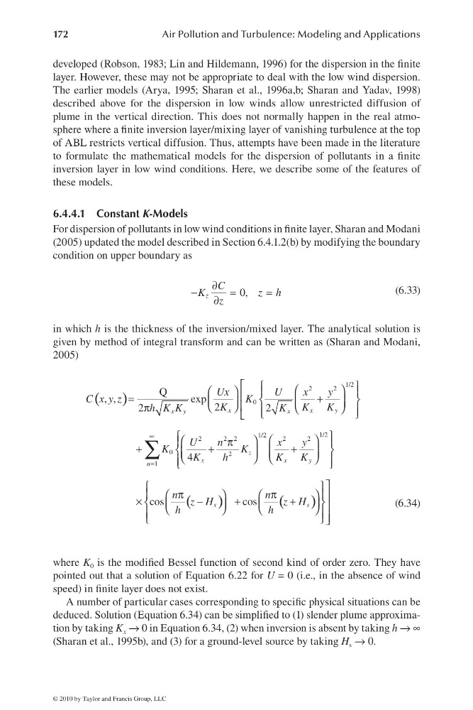
in which h is the thickness of the inversion/mixed layer. The analytical solution is
given by method of integral transform and can be written as (Sharan and Modani,
2005)
( )
(
)
(
)
∞
=
⎡ ⎧
⎫
⎛
⎞
⎛
⎞
⎪
⎪
⎢
=
+
⎨
⎬
⎜
⎟
⎜
⎟
⎢
⎝
⎠
π
⎝
⎠
⎪
⎪
⎩
⎭
⎣
⎧
⎫
⎛
⎞
⎛
⎞
π
⎪
⎪
+
+
+
⎨
⎬
⎜
⎟
⎜
⎟
⎝
⎠ ⎝
⎠
⎪
⎪
⎩
⎭
⎤
⎧
⎫
π
π
⎪
⎪
⎛
⎞
⎛
⎞ ⎥
×
−
+
+
⎨
⎬
⎜
⎟
⎜
⎟ ⎥
⎝
⎠
⎝
⎠
⎪
⎪ ⎥
⎩
⎭ ⎦
∑
1/2
2
2
0
1/2
1/2
2
2 2
2
2
0
2
1
Q
, ,
exp
2
2
2
4
cos
cos
x
x
y
x y
x
z
x
x
y
n
s
s
Ux
U
x
y
C x y z
K
K
K
K
h K K
K
U
n
x
y
K
K
K
h
K
K
n
n
z H
z H
h
h
(6.34)
where K 0 is the modifi ed Bessel function of second kind of order zero. They have
pointed out that a solution of Equation 6.22 for U = 0 (i.e., in the absence of wind
speed) in fi nite layer does not exist.
A number of particular cases corresponding to specifi c physical situations can be
deduced. Solution (Equation 6.34) can be simplifi ed to (1) slender plume approximation by taking K x → 0 in Equation 6.34, (2) when inversion is absent by taking h → ∞
(Sharan et al., 1995b), and (3) for a ground-level source by taking H s → 0.
© 2010 by Taylor and Francis Group, LLC
Air Pollution and Turbulence: Modeling and Applications
developed (Robson, 1983; Lin and Hildemann, 1996) for the dispersion in the fi nite
layer. However, these may not be appropriate to deal with the low wind dispersion.
The earlier models (Arya, 1995; Sharan et al., 1996a,b; Sharan and Yadav, 1998)
described above for the dispersion in low winds allow unrestricted diffusion of
plume in the vertical direction. This does not normally happen in the real atmosphere where a fi nite inversion layer/mixing layer of vanishing turbulence at the top
of ABL restricts vertical diffusion. Thus, attempts have been made in the literature
to formulate the mathematical models for the dispersion of pollutants in a fi nite
inversion layer in low wind conditions. Here, we describe some of the features of
these models.
6.4.4.1 Constant K-Models
For dispersion of pollutants in low wind conditions in fi nite layer, Sharan and Modani
(2005) updated the model described in Section 6.4.1.2(b) by modifying the boundary
condition on upper boundary as
∂
−
=
=
∂
0,
z
C
K
z h
z
(6.33)
in which h is the thickness of the inversion/mixed layer. The analytical solution is
given by method of integral transform and can be written as (Sharan and Modani,
2005)
( )
(
)
(
)
∞
=
⎡ ⎧
⎫
⎛
⎞
⎛
⎞
⎪
⎪
⎢
=
+
⎨
⎬
⎜
⎟
⎜
⎟
⎢
⎝
⎠
π
⎝
⎠
⎪
⎪
⎩
⎭
⎣
⎧
⎫
⎛
⎞
⎛
⎞
π
⎪
⎪
+
+
+
⎨
⎬
⎜
⎟
⎜
⎟
⎝
⎠ ⎝
⎠
⎪
⎪
⎩
⎭
⎤
⎧
⎫
π
π
⎪
⎪
⎛
⎞
⎛
⎞ ⎥
×
−
+
+
⎨
⎬
⎜
⎟
⎜
⎟ ⎥
⎝
⎠
⎝
⎠
⎪
⎪ ⎥
⎩
⎭ ⎦
∑
1/2
2
2
0
1/2
1/2
2
2 2
2
2
0
2
1
Q
, ,
exp
2
2
2
4
cos
cos
x
x
y
x y
x
z
x
x
y
n
s
s
Ux
U
x
y
C x y z
K
K
K
K
h K K
K
U
n
x
y
K
K
K
h
K
K
n
n
z H
z H
h
h
(6.34)
where K 0 is the modifi ed Bessel function of second kind of order zero. They have
pointed out that a solution of Equation 6.22 for U = 0 (i.e., in the absence of wind
speed) in fi nite layer does not exist.
A number of particular cases corresponding to specifi c physical situations can be
deduced. Solution (Equation 6.34) can be simplifi ed to (1) slender plume approximation by taking K x → 0 in Equation 6.34, (2) when inversion is absent by taking h → ∞
(Sharan et al., 1995b), and (3) for a ground-level source by taking H s → 0.
© 2010 by Taylor and Francis Group, LLC