

Analytical Models for the Dispersion of Pollutants in Low Wind Conditions 173
6.4.4.2 Variable K-Models
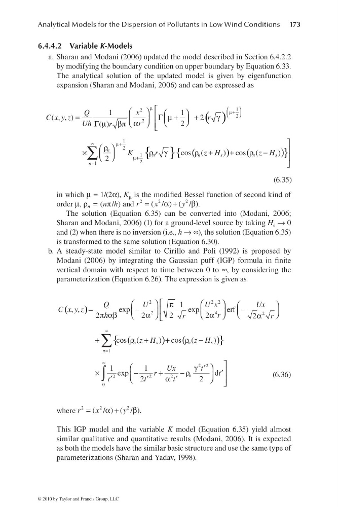
a. Sharan and Modani (2006) updated the model described in Section 6.4.2.2
by modifying the boundary condition on upper boundary by Equation 6.33.
The analytical solution of the updated model is given by eigenfunction
expansion (Sharan and Modani, 2006) and can be expressed as
( )
{ } (
)
(
)
{
}
1
2
2
2
1
2
1
2
1
1
1
( , , )
2
2
( )
cos (
) cos (
)
2
n
n
n
s
n
s
n
Q
x
C x y z
r
Uh
r
r
K
r
z H
z H
μ
⎛
⎞
μ+
⎜
⎟
⎝
⎠
∞
μ+
μ+
=
⎡
⎛
⎞
⎛
⎞
⎢
=
Γ μ +
+
γ
⎜
⎟
⎜
⎟
⎝
⎠
α
⎝
⎠
Γ μ βπ
⎢ ⎣
⎤
ρ
⎛ ⎞
⎥
×
ρ γ
ρ +
+
ρ −
⎜ ⎟
⎝ ⎠
⎥
⎦
∑
(6.35)
in which μ = 1/(2α), K μ is the modifi ed Bessel function of second kind of
order μ, ρ = π
( / )
n
n h and =
α +
β
2
2
2
( / ) ( / )
r
x
y
.
The solution (Equation 6.35) can be converted into (Modani, 2006;
Sharan and Modani, 2006) (1) for a ground-level source by taking H s → 0
and (2) when there is no inversion (i.e., h → ∞), the solution (Equation 6.35)
is transformed to the same solution (Equation 6.30).
b. A steady-state model similar to Cirillo and Poli (1992) is proposed by
Modani (2006) by integrating the Gaussian puff (IGP) formula in fi nite
vertical domain with respect to time between 0 to ∞, by considering the
parameterization (Equation 6.26). The expression is given as
(
)
(
)
(
)
{
}
2
2 2
2
4
2
1
2 2
2
2
2
0
1
, ,
exp
exp
erf
2
2
2
2
2
cos (
) cos (
)
1
1
exp
d
2
2
n
s
n
s
n
n
Q
U
Ux
U x
C x y z
h
r
r
r
z H
z H
Ux
t
r
t
t
t
t
∞
=
∞
⎡
⎛
⎞
⎛
⎞
π
⎛
⎞
=
−
−
⎜
⎟
⎢
⎜
⎟
⎜
⎟
⎝
⎠
π αβ
α
α
⎝
⎠
⎝
⎠
α
⎣
+
ρ +
+
ρ −
⎤
⎛
⎞
γ ′
⎥
×
−
+
−ρ
′
⎜
⎟
α
′
′
′
⎝
⎠ ⎥ ⎦
∑
∫
(6.36)
where =
α +
β
2
2
2
( / ) ( / ).
r
x
y
This IGP model and the variable K model (Equation 6.35) yield almost
similar qualitative and quantitative results (Modani, 2006). It is expected
as both the models have the similar basic structure and use the same type of
parameterizations (Sharan and Yadav, 1998).
© 2010 by Taylor and Francis Group, LLC
6.4.4.2 Variable K-Models
a. Sharan and Modani (2006) updated the model described in Section 6.4.2.2
by modifying the boundary condition on upper boundary by Equation 6.33.
The analytical solution of the updated model is given by eigenfunction
expansion (Sharan and Modani, 2006) and can be expressed as
( )
{ } (
)
(
)
{
}
1
2
2
2
1
2
1
2
1
1
1
( , , )
2
2
( )
cos (
) cos (
)
2
n
n
n
s
n
s
n
Q
x
C x y z
r
Uh
r
r
K
r
z H
z H
μ
⎛
⎞
μ+
⎜
⎟
⎝
⎠
∞
μ+
μ+
=
⎡
⎛
⎞
⎛
⎞
⎢
=
Γ μ +
+
γ
⎜
⎟
⎜
⎟
⎝
⎠
α
⎝
⎠
Γ μ βπ
⎢ ⎣
⎤
ρ
⎛ ⎞
⎥
×
ρ γ
ρ +
+
ρ −
⎜ ⎟
⎝ ⎠
⎥
⎦
∑
(6.35)
in which μ = 1/(2α), K μ is the modifi ed Bessel function of second kind of
order μ, ρ = π
( / )
n
n h and =
α +
β
2
2
2
( / ) ( / )
r
x
y
.
The solution (Equation 6.35) can be converted into (Modani, 2006;
Sharan and Modani, 2006) (1) for a ground-level source by taking H s → 0
and (2) when there is no inversion (i.e., h → ∞), the solution (Equation 6.35)
is transformed to the same solution (Equation 6.30).
b. A steady-state model similar to Cirillo and Poli (1992) is proposed by
Modani (2006) by integrating the Gaussian puff (IGP) formula in fi nite
vertical domain with respect to time between 0 to ∞, by considering the
parameterization (Equation 6.26). The expression is given as
(
)
(
)
(
)
{
}
2
2 2
2
4
2
1
2 2
2
2
2
0
1
, ,
exp
exp
erf
2
2
2
2
2
cos (
) cos (
)
1
1
exp
d
2
2
n
s
n
s
n
n
Q
U
Ux
U x
C x y z
h
r
r
r
z H
z H
Ux
t
r
t
t
t
t
∞
=
∞
⎡
⎛
⎞
⎛
⎞
π
⎛
⎞
=
−
−
⎜
⎟
⎢
⎜
⎟
⎜
⎟
⎝
⎠
π αβ
α
α
⎝
⎠
⎝
⎠
α
⎣
+
ρ +
+
ρ −
⎤
⎛
⎞
γ ′
⎥
×
−
+
−ρ
′
⎜
⎟
α
′
′
′
⎝
⎠ ⎥ ⎦
∑
∫
(6.36)
where =
α +
β
2
2
2
( / ) ( / ).
r
x
y
This IGP model and the variable K model (Equation 6.35) yield almost
similar qualitative and quantitative results (Modani, 2006). It is expected
as both the models have the similar basic structure and use the same type of
parameterizations (Sharan and Yadav, 1998).
© 2010 by Taylor and Francis Group, LLC