

Analytical Models for the Dispersion of Pollutants in Low Wind Conditions 163
(
)
(
)
⎡
⎤
⎛
⎞
−
=
−
+
⎢
⎥
⎜
⎟
π σ σ σ
σ
σ
⎝
⎠
⎢
⎥
⎣
⎦
⎧
⎫
⎡
⎤
⎡
⎤
−
+
⎪
⎪
⎢
⎥
⎢
⎥
×
−
+
−
⎨
⎬
σ
σ
⎢
⎥
⎢
⎥
⎪
⎪
⎣
⎦
⎣
⎦
⎩
⎭
3/2
(
)
( , , , )
exp
(2 )
2
2
exp
exp
2
2
2
2
2
2
x y z
x
y
2
2
s
s
2
2
z
z
q
x U t
y
C x y z t
z H
z H
(6.14)
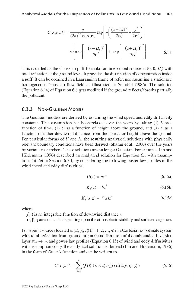
This is called as the Gaussian puff formula for an elevated source at (0, 0, H s ) with
total refl ection at the ground level. It provides the distribution of concentration inside
a puff. It can be obtained in a Lagrangian frame of reference assuming a stationary,
homogeneous Gaussian fl ow fi eld as illustrated in Seinfeld (1986). The solution
(Equation 6.14) of Equation 6.8 gets modifi ed if the ground refl ects/absorbs partially
the pollutant.
6.3.3 NON-GAUSSIAN MODELS
The Gaussian models are derived by assuming the wind speed and eddy diffusivity
constants. This assumption has been relaxed over the years by taking (1) K as a
function of time, (2) U as a function of height above the ground, and (3) K as a
function of either downwind distance from the source or height above the ground.
For particular forms of U and K, the resulting analytical solutions with physically
relevant boundary conditions have been derived (Sharan et al., 2003) over the years
by various researchers. These solutions are no longer Gaussian. For example, Lin and
Hildemann (1996) described an analytical solution for Equation 6.1 with assumptions (a)–(e) in Section 6.3.1, by considering the following power-law profi les of the
wind speed and eddy diffusivities:
α
=
( )
U z
az
(6.15a)
β
=
( )
z
K z
bz
(6.15b)
γ
=
( , )
( )
y
K x z
f x z
(6.15c)
where
f(x) is an integrable function of downwind distance x
α, β, γ are constants depending upon the atmospheric stability and surface roughness
For n point sources located at (x s
i , y s
i , z s
i ) (i = 1, 2, …, n) in a Cartesian coordinate system
with total refl ection from ground at z = 0 and from top of the unbounded inversion
layer at z → ∞, and power-law profi les (Equation 6.15) of wind and eddy diffusivities
with assumption α = γ, the analytical solution is derived (Lin and Hildemann, 1996)
in the form of Green’s function and can be written as
=
= ∑
1
( , , )
( , ; , ) ( , ; , )
n
i i
i
i
i
i
i
z
S
S
y
S S
i
C x y z
Q G x z x z G x y x y
(6.16)
© 2010 by Taylor and Francis Group, LLC
(
)
(
)
⎡
⎤
⎛
⎞
−
=
−
+
⎢
⎥
⎜
⎟
π σ σ σ
σ
σ
⎝
⎠
⎢
⎥
⎣
⎦
⎧
⎫
⎡
⎤
⎡
⎤
−
+
⎪
⎪
⎢
⎥
⎢
⎥
×
−
+
−
⎨
⎬
σ
σ
⎢
⎥
⎢
⎥
⎪
⎪
⎣
⎦
⎣
⎦
⎩
⎭
3/2
(
)
( , , , )
exp
(2 )
2
2
exp
exp
2
2
2
2
2
2
x y z
x
y
2
2
s
s
2
2
z
z
q
x U t
y
C x y z t
z H
z H
(6.14)
This is called as the Gaussian puff formula for an elevated source at (0, 0, H s ) with
total refl ection at the ground level. It provides the distribution of concentration inside
a puff. It can be obtained in a Lagrangian frame of reference assuming a stationary,
homogeneous Gaussian fl ow fi eld as illustrated in Seinfeld (1986). The solution
(Equation 6.14) of Equation 6.8 gets modifi ed if the ground refl ects/absorbs partially
the pollutant.
6.3.3 NON-GAUSSIAN MODELS
The Gaussian models are derived by assuming the wind speed and eddy diffusivity
constants. This assumption has been relaxed over the years by taking (1) K as a
function of time, (2) U as a function of height above the ground, and (3) K as a
function of either downwind distance from the source or height above the ground.
For particular forms of U and K, the resulting analytical solutions with physically
relevant boundary conditions have been derived (Sharan et al., 2003) over the years
by various researchers. These solutions are no longer Gaussian. For example, Lin and
Hildemann (1996) described an analytical solution for Equation 6.1 with assumptions (a)–(e) in Section 6.3.1, by considering the following power-law profi les of the
wind speed and eddy diffusivities:
α
=
( )
U z
az
(6.15a)
β
=
( )
z
K z
bz
(6.15b)
γ
=
( , )
( )
y
K x z
f x z
(6.15c)
where
f(x) is an integrable function of downwind distance x
α, β, γ are constants depending upon the atmospheric stability and surface roughness
For n point sources located at (x s
i , y s
i , z s
i ) (i = 1, 2, …, n) in a Cartesian coordinate system
with total refl ection from ground at z = 0 and from top of the unbounded inversion
layer at z → ∞, and power-law profi les (Equation 6.15) of wind and eddy diffusivities
with assumption α = γ, the analytical solution is derived (Lin and Hildemann, 1996)
in the form of Green’s function and can be written as
=
= ∑
1
( , , )
( , ; , ) ( , ; , )
n
i i
i
i
i
i
i
z
S
S
y
S S
i
C x y z
Q G x z x z G x y x y
(6.16)
© 2010 by Taylor and Francis Group, LLC