

162
Air Pollution and Turbulence: Modeling and Applications
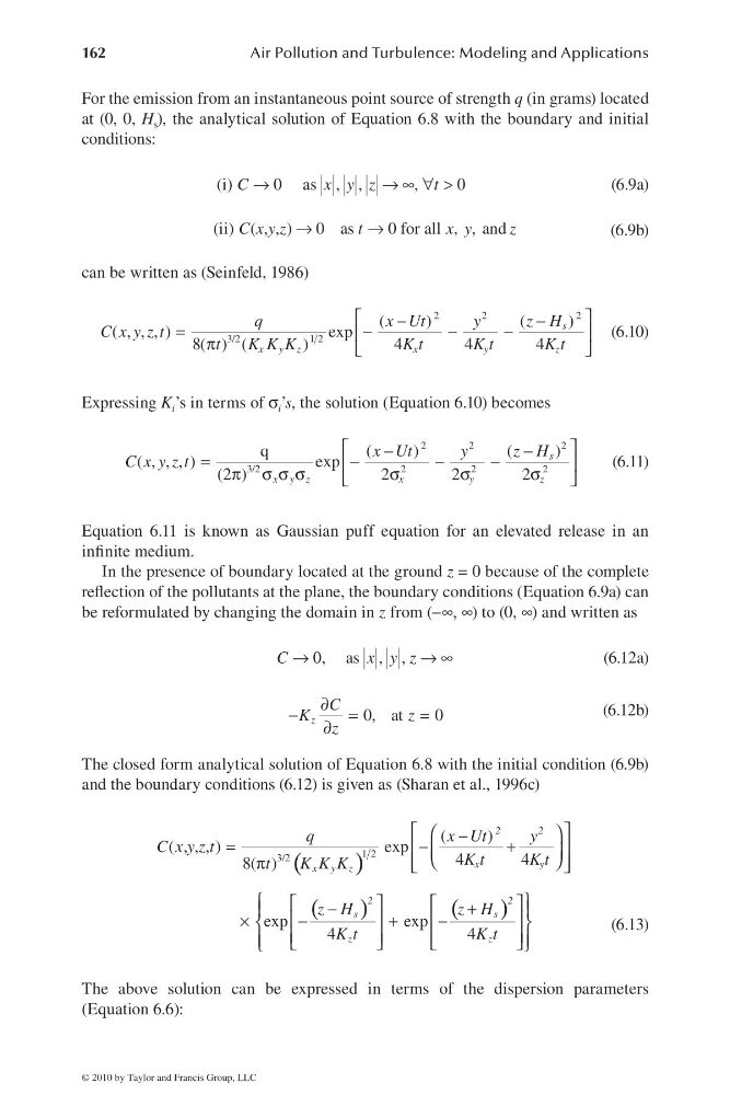
For the emission from an instantaneous point source of strength q (in grams) located
at (0, 0, H s ), the analytical solution of Equation 6.8 with the boundary and initial
conditions:
→
→ ∞∀>
(i)
0 as , ,
,
0
C
x y z
t
(6.9a)
→
→
(ii) ( , , ) 0 as
0 for all , , and
C x y z
t
x y
z
(6.9b)
can be written as (Seinfeld, 1986)
⎡
⎤
−
−
=
−
−
−
⎢
⎥
π
⎣
⎦
2
2
2
3/2
1 2
(
)
(
)
( , , , )
exp
8( ) (
)
4
4
4
s
x
y z
x
y
z
q
x U t
y
z H
C x y z t
t
K K K
K t
K t
Kt
(6.10)
Expressing K i ’s in terms of σ i ’s, the solution (Equation 6.10) becomes
⎡
⎤
−
−
=
−
−
−
⎢
⎥
π σσσ
σ
σ
σ
⎣
⎦
2
2
2
3/2
2
2
2
q
(
)
(
)
( , , , )
exp
( 2 )
2
2
2
s
x y z
x
y
z
x Ut
y
z H
C x y z t
(6.11)
Equation 6.11 is known as Gaussian puff equation for an elevated release in an
infi nite medium.
In the presence of boundary located at the ground z = 0 because of the complete
refl ection of the pollutants at the plane, the boundary conditions (Equation 6.9a) can
be reformulated by changing the domain in z from (−∞, ∞) to (0, ∞) and written as
→
→ ∞
0, as , ,
C
x y z
(6.12a)
∂
−
=
∂
0, at = 0
z
C
K
z
z
(6.12b)
The closed form analytical solution of Equation 6.8 with the initial condition (6.9b)
and the boundary conditions (6.12) is given as (Sharan et al., 1996c)
(
)
(
)
(
)
⎡
⎤
⎛
⎞
−
=
−
+
⎢
⎥
⎜
⎟
⎝
⎠
π
⎢
⎥
⎣
⎦
⎧
⎫
⎡
⎤
⎡
⎤
−
+
⎪
⎪
⎢
⎥
⎢
⎥
×
−
+
−
⎨
⎬
⎢
⎥
⎢
⎥
⎪
⎪
⎣
⎦
⎣
⎦
⎩
⎭
1 2
3/2
(
)
( , , , )
exp
4
4
8( )
exp
exp
4
4
2
2
x
y
x y z
2
2
s
s
z
z
q
xU t
y
C x y z t
K t
K t
t
K K K
z H
z H
K t
K t
(6.13)
The above solution can be expressed in terms of the dispersion parameters
(Equation 6.6):
© 2010 by Taylor and Francis Group, LLC
Air Pollution and Turbulence: Modeling and Applications
For the emission from an instantaneous point source of strength q (in grams) located
at (0, 0, H s ), the analytical solution of Equation 6.8 with the boundary and initial
conditions:
→
→ ∞∀>
(i)
0 as , ,
,
0
C
x y z
t
(6.9a)
→
→
(ii) ( , , ) 0 as
0 for all , , and
C x y z
t
x y
z
(6.9b)
can be written as (Seinfeld, 1986)
⎡
⎤
−
−
=
−
−
−
⎢
⎥
π
⎣
⎦
2
2
2
3/2
1 2
(
)
(
)
( , , , )
exp
8( ) (
)
4
4
4
s
x
y z
x
y
z
q
x U t
y
z H
C x y z t
t
K K K
K t
K t
Kt
(6.10)
Expressing K i ’s in terms of σ i ’s, the solution (Equation 6.10) becomes
⎡
⎤
−
−
=
−
−
−
⎢
⎥
π σσσ
σ
σ
σ
⎣
⎦
2
2
2
3/2
2
2
2
q
(
)
(
)
( , , , )
exp
( 2 )
2
2
2
s
x y z
x
y
z
x Ut
y
z H
C x y z t
(6.11)
Equation 6.11 is known as Gaussian puff equation for an elevated release in an
infi nite medium.
In the presence of boundary located at the ground z = 0 because of the complete
refl ection of the pollutants at the plane, the boundary conditions (Equation 6.9a) can
be reformulated by changing the domain in z from (−∞, ∞) to (0, ∞) and written as
→
→ ∞
0, as , ,
C
x y z
(6.12a)
∂
−
=
∂
0, at = 0
z
C
K
z
z
(6.12b)
The closed form analytical solution of Equation 6.8 with the initial condition (6.9b)
and the boundary conditions (6.12) is given as (Sharan et al., 1996c)
(
)
(
)
(
)
⎡
⎤
⎛
⎞
−
=
−
+
⎢
⎥
⎜
⎟
⎝
⎠
π
⎢
⎥
⎣
⎦
⎧
⎫
⎡
⎤
⎡
⎤
−
+
⎪
⎪
⎢
⎥
⎢
⎥
×
−
+
−
⎨
⎬
⎢
⎥
⎢
⎥
⎪
⎪
⎣
⎦
⎣
⎦
⎩
⎭
1 2
3/2
(
)
( , , , )
exp
4
4
8( )
exp
exp
4
4
2
2
x
y
x y z
2
2
s
s
z
z
q
xU t
y
C x y z t
K t
K t
t
K K K
z H
z H
K t
K t
(6.13)
The above solution can be expressed in terms of the dispersion parameters
(Equation 6.6):
© 2010 by Taylor and Francis Group, LLC