

Mathematical Air Pollution Models: Eulerian Models
143
Gaussian models can simulate complex, area or volume sources, both by the
spatial integration of the contribution of emissions (made possible because Gaussian
models are linear to emissions), and, to obviate the diffi culties of integration, by
using special algorithms.
In practice, they can be relatively easy to use, and can be applied in numerous
conditions (e.g., isolated sources, cities, road traffi c, complex terrain). Moreover,
bearing in mind that in practical applications, meteorological data are not generally
available at both ground level and aloft at high temporal/spatial resolution, their
performances are not poorer than those of other models. For these reasons, most
operative models are based on the Gaussian approach.
The Gaussian model can be modifi ed so as to extend its applicability to nonstationary and nonhomogeneous conditions, as well as to more complex orography. In
particular, the breaking down of the plume into puffs has permitted the simulation of
pollutant dispersion in pseudostationary conditions. Such models, illustrated below,
decompose the plume into puffs, whose characteristics evolve in time and space
together with the changing meteorological and emission conditions.
The various versions of Gaussian models essentially differ in the techniques
utilized to calculate the “sigmas” as a function of atmospheric stability and the
downwind distance from the emission source.
5.4 SEMIEMPIRICAL EXPRESSIONS OF THE s
Several schemas exist for the calculation of σ y and σ z as functions of stability classes
and of the downwind distance from the source.
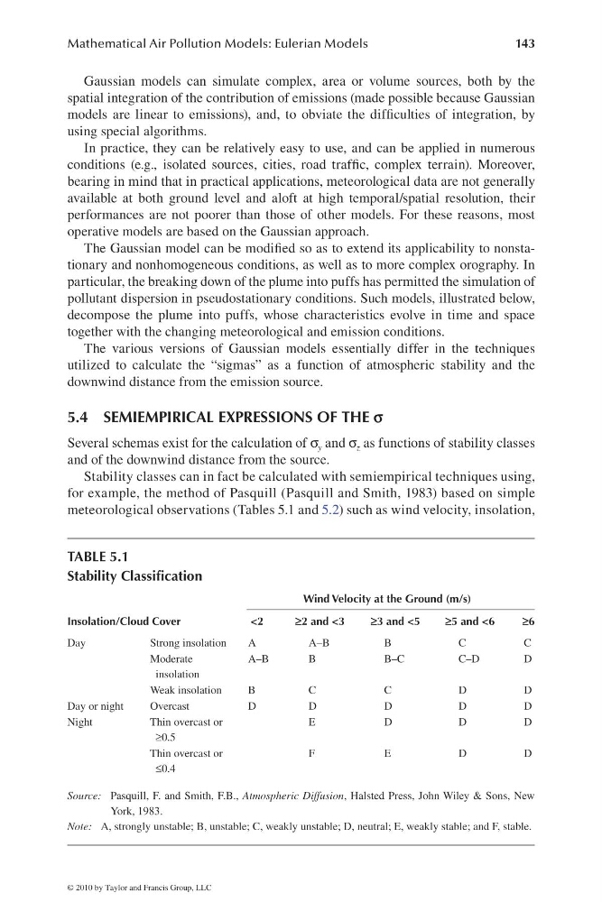
Stability classes can in fact be calculated with semiempirical techniques using,
for example, the method of Pasquill (Pasquill and Smith, 1983) based on simple
meteorological observations (Tables 5.1 and 5.2) such as wind velocity, insolation,
TABLE 5.1
Stability Classifi cation
Wind Velocity at the Ground (m/s)
Insolation/Cloud Cover
<2
≥2 and <3
≥3 and <5
≥5 and <6
≥6
Day
Strong insolation
A
A–B
B
C
C
Moderate
insolation
A–B
B
B–C
C–D
D
Weak insolation
B
C
C
D
D
Day or night
Overcast
D
D
D
D
D
Night
Thin overcast or
≥0.5
E
D
D
D
Thin overcast or
≤0.4
F
E
D
D
Source: Pasquill, F. and Smith, F.B., Atmospheric Diffusion, Halsted Press, John Wiley & Sons, New
York, 1983.
Note: A, strongly unstable; B, unstable; C, weakly unstable; D, neutral; E, weakly stable; and F, stable.
© 2010 by Taylor and Francis Group, LLC
143
Gaussian models can simulate complex, area or volume sources, both by the
spatial integration of the contribution of emissions (made possible because Gaussian
models are linear to emissions), and, to obviate the diffi culties of integration, by
using special algorithms.
In practice, they can be relatively easy to use, and can be applied in numerous
conditions (e.g., isolated sources, cities, road traffi c, complex terrain). Moreover,
bearing in mind that in practical applications, meteorological data are not generally
available at both ground level and aloft at high temporal/spatial resolution, their
performances are not poorer than those of other models. For these reasons, most
operative models are based on the Gaussian approach.
The Gaussian model can be modifi ed so as to extend its applicability to nonstationary and nonhomogeneous conditions, as well as to more complex orography. In
particular, the breaking down of the plume into puffs has permitted the simulation of
pollutant dispersion in pseudostationary conditions. Such models, illustrated below,
decompose the plume into puffs, whose characteristics evolve in time and space
together with the changing meteorological and emission conditions.
The various versions of Gaussian models essentially differ in the techniques
utilized to calculate the “sigmas” as a function of atmospheric stability and the
downwind distance from the emission source.
5.4 SEMIEMPIRICAL EXPRESSIONS OF THE s
Several schemas exist for the calculation of σ y and σ z as functions of stability classes
and of the downwind distance from the source.
Stability classes can in fact be calculated with semiempirical techniques using,
for example, the method of Pasquill (Pasquill and Smith, 1983) based on simple
meteorological observations (Tables 5.1 and 5.2) such as wind velocity, insolation,
TABLE 5.1
Stability Classifi cation
Wind Velocity at the Ground (m/s)
Insolation/Cloud Cover
<2
≥2 and <3
≥3 and <5
≥5 and <6
≥6
Day
Strong insolation
A
A–B
B
C
C
Moderate
insolation
A–B
B
B–C
C–D
D
Weak insolation
B
C
C
D
D
Day or night
Overcast
D
D
D
D
D
Night
Thin overcast or
≥0.5
E
D
D
D
Thin overcast or
≤0.4
F
E
D
D
Source: Pasquill, F. and Smith, F.B., Atmospheric Diffusion, Halsted Press, John Wiley & Sons, New
York, 1983.
Note: A, strongly unstable; B, unstable; C, weakly unstable; D, neutral; E, weakly stable; and F, stable.
© 2010 by Taylor and Francis Group, LLC