

Parameterization of Convective Boundary Layer Turbulence and Clouds
111
equations can be obtained using Reynolds decomposition and averaging, with three
important terms in the r.h.s.: a term representing the production of variance, a second
term representing the transport, and a third term the dissipation of variance.
A simplifi cation of these prognostic equations is often used as a fi rst approximation, where steady state is assumed and the third-order transport term is neglected.
This simplifi cation allows to go from a partial differential equation to an algebraic
equation in determining the variance as a function of the sub-grid vertical fl ux and
the vertical gradient of the mean temperature or water variable.
The major issue with PDF-based methods is how to determine the characteristics
of the PDF itself. As briefl y discussed above, in terms of the model, it is possible
(even if not always feasible), using Reynolds decomposition and averaging, to obtain
equations for the variance and for the skewness of the PDF. What is still unclear
is how the PDFs look like for different physical situations and different types of
clouds.
Aircraft observations (e.g., Larson et al. 2001) and LES models (e.g., Cuijpers
and Bechtold 1994) support the idea that for most stratus clouds, a Gaussian PDF
is a realistic approximation. However, for cumulus clouds, the skewness of the PDF
may well play an important role in determining the cloud properties. For example,
Bougeault (1981) analyzed the results produced by a 3D LES model, in order to
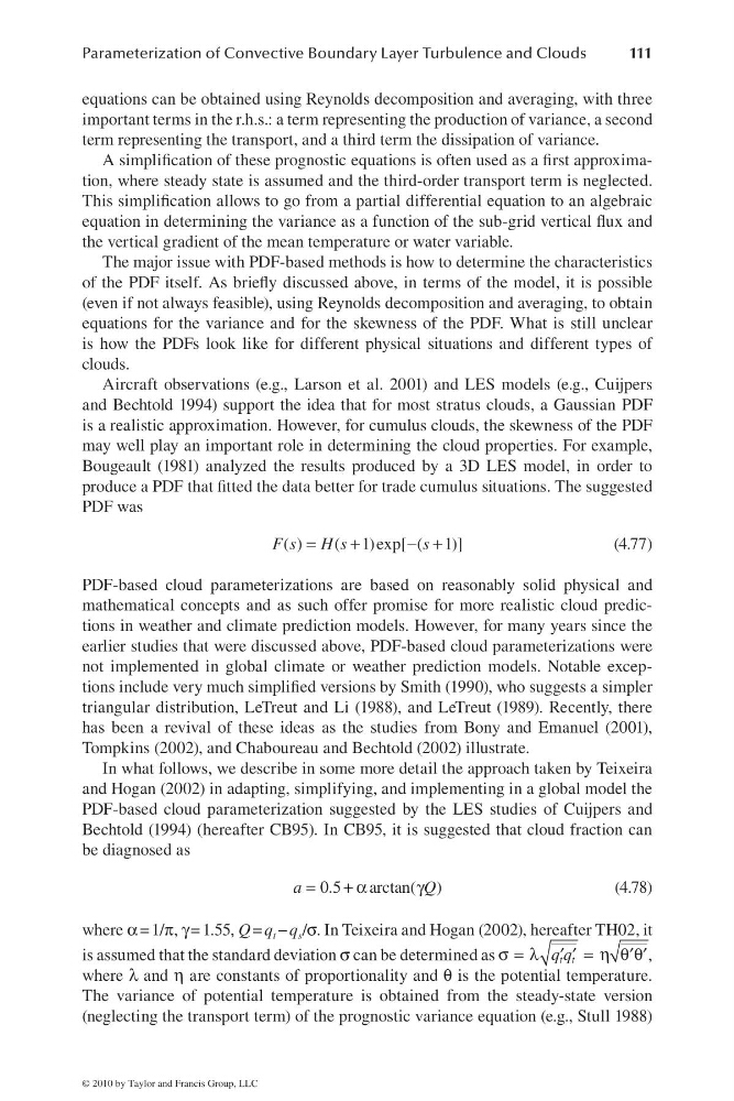
produce a PDF that fi tted the data better for trade cumulus situations. The suggested
PDF was
( )
( 1)exp[ ( 1)]
F s H s
s
=
+
− +
(4.77)
PDF-based cloud parameterizations are based on reasonably solid physical and
mathematical concepts and as such offer promise for more realistic cloud predictions in weather and climate prediction models. However, for many years since the
earlier studies that were discussed above, PDF-based cloud parameterizations were
not implemented in global climate or weather prediction models. Notable exceptions include very much simplifi ed versions by Smith (1990), who suggests a simpler
triangular distribution, LeTreut and Li (1988), and LeTreut (1989). Recently, there
has been a revival of these ideas as the studies from Bony and Emanuel (2001),
Tompkins (2002), and Chaboureau and Bechtold (2002) illustrate.
In what follows, we describe in some more detail the approach taken by Teixeira
and Hogan (2002) in adapting, simplifying, and implementing in a global model the
PDF-based cloud parameterization suggested by the LES studies of Cuijpers and
Bechtold (1994) (hereafter CB95). In CB95, it is suggested that cloud fraction can
be diagnosed as
0.5
arctan( )
a
Q
=
+α
γ
(4.78)
where α = 1/π, γ = 1.55, Q = q t − q s /σ. In Teixeira and Hogan (2002), hereafter TH02, it
is assumed that the standard deviation σ can be determined as σ = λ
= η θ θ
′ ′
′ ′
t t
q q
,
where λ and η are constants of proportionality and θ is the potential temperature.
The variance of potential temperature is obtained from the steady-state version
(neglecting the transport term) of the prognostic variance equation (e.g., Stull 1988)
© 2010 by Taylor and Francis Group, LLC
111
equations can be obtained using Reynolds decomposition and averaging, with three
important terms in the r.h.s.: a term representing the production of variance, a second
term representing the transport, and a third term the dissipation of variance.
A simplifi cation of these prognostic equations is often used as a fi rst approximation, where steady state is assumed and the third-order transport term is neglected.
This simplifi cation allows to go from a partial differential equation to an algebraic
equation in determining the variance as a function of the sub-grid vertical fl ux and
the vertical gradient of the mean temperature or water variable.
The major issue with PDF-based methods is how to determine the characteristics
of the PDF itself. As briefl y discussed above, in terms of the model, it is possible
(even if not always feasible), using Reynolds decomposition and averaging, to obtain
equations for the variance and for the skewness of the PDF. What is still unclear
is how the PDFs look like for different physical situations and different types of
clouds.
Aircraft observations (e.g., Larson et al. 2001) and LES models (e.g., Cuijpers
and Bechtold 1994) support the idea that for most stratus clouds, a Gaussian PDF
is a realistic approximation. However, for cumulus clouds, the skewness of the PDF
may well play an important role in determining the cloud properties. For example,
Bougeault (1981) analyzed the results produced by a 3D LES model, in order to
produce a PDF that fi tted the data better for trade cumulus situations. The suggested
PDF was
( )
( 1)exp[ ( 1)]
F s H s
s
=
+
− +
(4.77)
PDF-based cloud parameterizations are based on reasonably solid physical and
mathematical concepts and as such offer promise for more realistic cloud predictions in weather and climate prediction models. However, for many years since the
earlier studies that were discussed above, PDF-based cloud parameterizations were
not implemented in global climate or weather prediction models. Notable exceptions include very much simplifi ed versions by Smith (1990), who suggests a simpler
triangular distribution, LeTreut and Li (1988), and LeTreut (1989). Recently, there
has been a revival of these ideas as the studies from Bony and Emanuel (2001),
Tompkins (2002), and Chaboureau and Bechtold (2002) illustrate.
In what follows, we describe in some more detail the approach taken by Teixeira
and Hogan (2002) in adapting, simplifying, and implementing in a global model the
PDF-based cloud parameterization suggested by the LES studies of Cuijpers and
Bechtold (1994) (hereafter CB95). In CB95, it is suggested that cloud fraction can
be diagnosed as
0.5
arctan( )
a
Q
=
+α
γ
(4.78)
where α = 1/π, γ = 1.55, Q = q t − q s /σ. In Teixeira and Hogan (2002), hereafter TH02, it
is assumed that the standard deviation σ can be determined as σ = λ
= η θ θ
′ ′
′ ′
t t
q q
,
where λ and η are constants of proportionality and θ is the potential temperature.
The variance of potential temperature is obtained from the steady-state version
(neglecting the transport term) of the prognostic variance equation (e.g., Stull 1988)
© 2010 by Taylor and Francis Group, LLC