

110
Air Pollution and Turbulence: Modeling and Applications
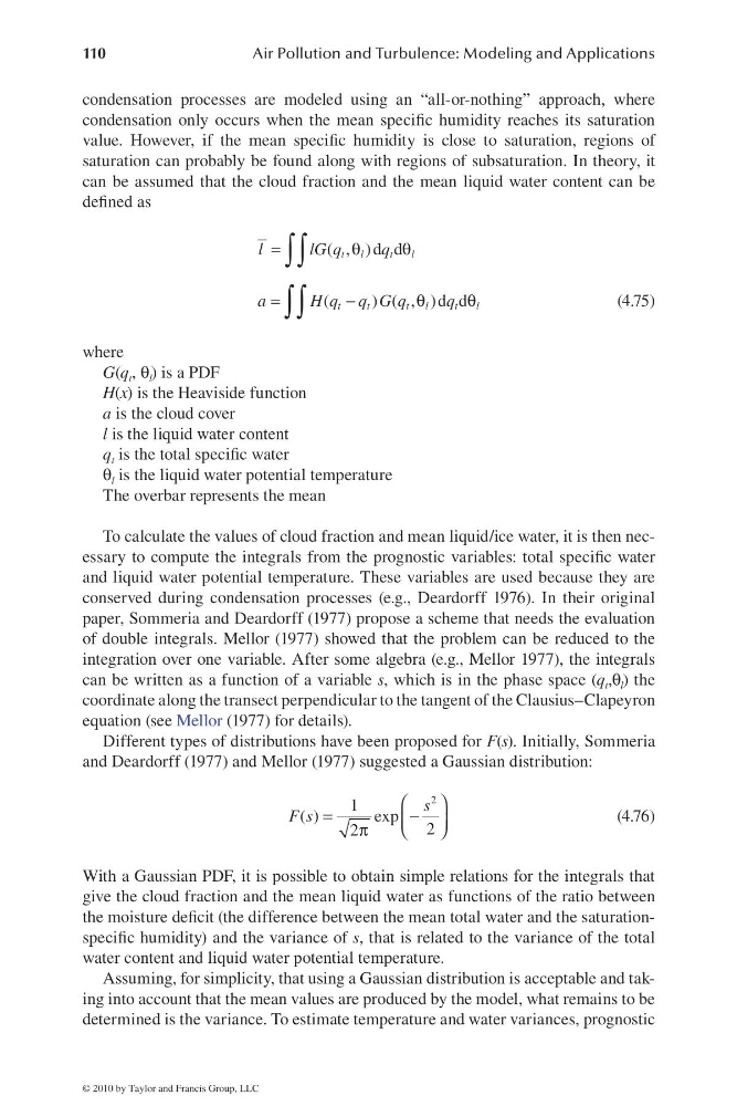
condensation processes are modeled using an “all-or-nothing” approach, where
condensation only occurs when the mean specifi c humidity reaches its saturation
value. However, if the mean specifi c humidity is close to saturation, regions of
saturation can probably be found along with regions of subsaturation. In theory, it
can be assumed that the cloud fraction and the mean liquid water content can be
defi ned as
=
θ
θ
=
−
θ
θ
∫∫
∫∫
( , )d d
(
) ( , )d d
t
l
t
l
t
t
t
l
t
l
l
lGq
q
a
H q q G q
q
(4.75)
where
G(q t , θ l ) is a PDF
H(x) is the Heaviside function
a is the cloud cover
l is the liquid water content
q t is the total specifi c water
θ l is the liquid water potential temperature
The overbar represents the mean
To calculate the values of cloud fraction and mean liquid/ice water, it is then necessary to compute the integrals from the prognostic variables: total specifi c water
and liquid water potential temperature. These variables are used because they are
conserved during condensation processes (e.g., Deardorff 1976). In their original
paper, Sommeria and Deardorff (1977) propose a scheme that needs the evaluation
of double integrals. Mellor (1977) showed that the problem can be reduced to the
integration over one variable. After some algebra (e.g., Mellor 1977), the integrals
can be written as a function of a variable s, which is in the phase space (q t ,θ l ) the
coordinate along the transect perpendicular to the tangent of the Clausius–Clapeyron
equation (see Mellor (1977) for details).
Different types of distributions have been proposed for F(s). Initially, Sommeria
and Deardorff (1977) and Mellor (1977) suggested a Gaussian distribution:
⎛
⎞
=
−
⎜
⎟
⎝
⎠
π
2
1
( )
exp
2
2
s
F s
(4.76)
With a Gaussian PDF, it is possible to obtain simple relations for the integrals that
give the cloud fraction and the mean liquid water as functions of the ratio between
the moisture defi cit (the difference between the mean total water and the saturationspecifi c humidity) and the variance of s, that is related to the variance of the total
water content and liquid water potential temperature.
Assuming, for simplicity, that using a Gaussian distribution is acceptable and taking into account that the mean values are produced by the model, what remains to be
determined is the variance. To estimate temperature and water variances, prognostic
© 2010 by Taylor and Francis Group, LLC
Air Pollution and Turbulence: Modeling and Applications
condensation processes are modeled using an “all-or-nothing” approach, where
condensation only occurs when the mean specifi c humidity reaches its saturation
value. However, if the mean specifi c humidity is close to saturation, regions of
saturation can probably be found along with regions of subsaturation. In theory, it
can be assumed that the cloud fraction and the mean liquid water content can be
defi ned as
=
θ
θ
=
−
θ
θ
∫∫
∫∫
( , )d d
(
) ( , )d d
t
l
t
l
t
t
t
l
t
l
l
lGq
q
a
H q q G q
q
(4.75)
where
G(q t , θ l ) is a PDF
H(x) is the Heaviside function
a is the cloud cover
l is the liquid water content
q t is the total specifi c water
θ l is the liquid water potential temperature
The overbar represents the mean
To calculate the values of cloud fraction and mean liquid/ice water, it is then necessary to compute the integrals from the prognostic variables: total specifi c water
and liquid water potential temperature. These variables are used because they are
conserved during condensation processes (e.g., Deardorff 1976). In their original
paper, Sommeria and Deardorff (1977) propose a scheme that needs the evaluation
of double integrals. Mellor (1977) showed that the problem can be reduced to the
integration over one variable. After some algebra (e.g., Mellor 1977), the integrals
can be written as a function of a variable s, which is in the phase space (q t ,θ l ) the
coordinate along the transect perpendicular to the tangent of the Clausius–Clapeyron
equation (see Mellor (1977) for details).
Different types of distributions have been proposed for F(s). Initially, Sommeria
and Deardorff (1977) and Mellor (1977) suggested a Gaussian distribution:
⎛
⎞
=
−
⎜
⎟
⎝
⎠
π
2
1
( )
exp
2
2
s
F s
(4.76)
With a Gaussian PDF, it is possible to obtain simple relations for the integrals that
give the cloud fraction and the mean liquid water as functions of the ratio between
the moisture defi cit (the difference between the mean total water and the saturationspecifi c humidity) and the variance of s, that is related to the variance of the total
water content and liquid water potential temperature.
Assuming, for simplicity, that using a Gaussian distribution is acceptable and taking into account that the mean values are produced by the model, what remains to be
determined is the variance. To estimate temperature and water variances, prognostic
© 2010 by Taylor and Francis Group, LLC