

108
Air Pollution and Turbulence: Modeling and Applications
The Slingo (1987) scheme is based on diagnostic relations between cloud fraction
and relative humidity. One of its main objectives was to be able to simulate stratocumulus clouds realistically. To be able to do that, the cloud fraction is also related
diagnostically to the strength of the BL inversion. This scheme is described in
Section 4.5.2.
The PDF-based parameterizations (e.g., Mellor 1977; Sommeria and Deardorff
1977) were not initially developed to be used in global models of the atmosphere
and its initial applications were cloud-resolving models of the atmospheric boundary
layer, followed by 1D BL models. Only later was this method applied to large-scale
models. This scheme is described in Section 4.5.3.
Only about a decade ago did prognostic cloud schemes started to be implemented
in global models. Until 1991, prognostic cloud schemes treated cloud fraction by
means of diagnostic relations (e.g., Sundqvist 1988). In Tiedtke (1991) a prognostic
equation for cloud fraction was proposed, but in this work only convective clouds
were considered. In Tiedtke (1993), a more complete parameterization with a prognostic cloud fraction equation was presented. This scheme is described in detail in
Section 4.5.4.
The prognostic cloud schemes based on the Sundqvist approach (e.g., Sundqvist
1988) have a prognostic variable for liquid/ice water only. These schemes are not
described here because they were not aimed at parameterizing BL clouds. Also,
Sundqvist’s approach of having a prognostic equation for the liquid/ice water content
and a diagnostic equation for the cloud fraction is believed to be less consistent.
To fi nalize this section, simplifi ed versions of the PDF-based and the prognostic
cloud parameterizations are discussed. In the following section, only the parts of the
cloud parameterizations that are relevant for the BL are discussed.
4.5.2 THE SLINGO DIAGNOSTIC CLOUD SCHEME
In this section, the scheme introduced by Slingo (1987) is described in the way it
was operational in the ECMWF model until 1995. This cloud scheme allows for four
cloud types: convective and three layer clouds (high, middle, and low level). Clouds
are computed at every model level using different relations depending on where they
are located in the vertical.
The convective clouds are computed whenever the convection scheme is active
and can fi ll any number of model layers. The convective cloud depth is determined
by the convection scheme. The convective clouds C c are determined from the convective precipitation rate P (mm day −1 ), C c = 0.4 min (0.8, 0.125 log e (P) − 1.5). The
cloud base and top heights are also derived from the convection scheme.
Two types of BL clouds are parameterized: clouds associated with extratropical
fronts and tropical disturbances and clouds that occur in relatively quiescent conditions and are directly associated with the boundary layer. The fi rst class of clouds are
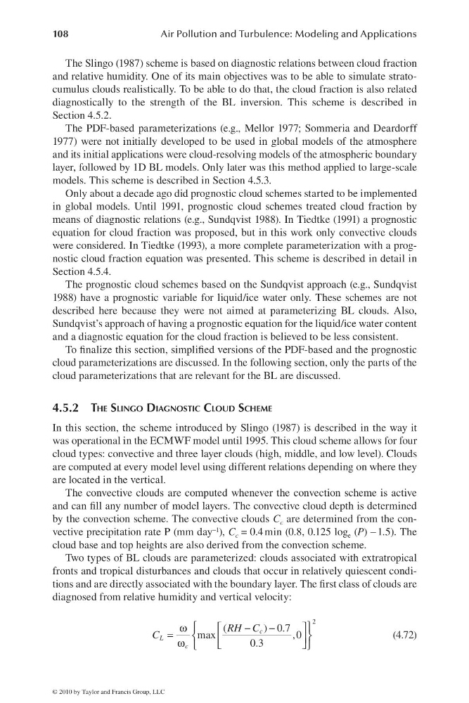
diagnosed from relative humidity and vertical velocity:
2
(
) 0.7
max
,0
0.3
c
L
c
RH C
C
⎧
⎫
ω
−
−
⎡
⎤
=
⎨
⎬
⎢
⎥
ω
⎣
⎦
⎩
⎭
(4.72)
© 2010 by Taylor and Francis Group, LLC
Air Pollution and Turbulence: Modeling and Applications
The Slingo (1987) scheme is based on diagnostic relations between cloud fraction
and relative humidity. One of its main objectives was to be able to simulate stratocumulus clouds realistically. To be able to do that, the cloud fraction is also related
diagnostically to the strength of the BL inversion. This scheme is described in
Section 4.5.2.
The PDF-based parameterizations (e.g., Mellor 1977; Sommeria and Deardorff
1977) were not initially developed to be used in global models of the atmosphere
and its initial applications were cloud-resolving models of the atmospheric boundary
layer, followed by 1D BL models. Only later was this method applied to large-scale
models. This scheme is described in Section 4.5.3.
Only about a decade ago did prognostic cloud schemes started to be implemented
in global models. Until 1991, prognostic cloud schemes treated cloud fraction by
means of diagnostic relations (e.g., Sundqvist 1988). In Tiedtke (1991) a prognostic
equation for cloud fraction was proposed, but in this work only convective clouds
were considered. In Tiedtke (1993), a more complete parameterization with a prognostic cloud fraction equation was presented. This scheme is described in detail in
Section 4.5.4.
The prognostic cloud schemes based on the Sundqvist approach (e.g., Sundqvist
1988) have a prognostic variable for liquid/ice water only. These schemes are not
described here because they were not aimed at parameterizing BL clouds. Also,
Sundqvist’s approach of having a prognostic equation for the liquid/ice water content
and a diagnostic equation for the cloud fraction is believed to be less consistent.
To fi nalize this section, simplifi ed versions of the PDF-based and the prognostic
cloud parameterizations are discussed. In the following section, only the parts of the
cloud parameterizations that are relevant for the BL are discussed.
4.5.2 THE SLINGO DIAGNOSTIC CLOUD SCHEME
In this section, the scheme introduced by Slingo (1987) is described in the way it
was operational in the ECMWF model until 1995. This cloud scheme allows for four
cloud types: convective and three layer clouds (high, middle, and low level). Clouds
are computed at every model level using different relations depending on where they
are located in the vertical.
The convective clouds are computed whenever the convection scheme is active
and can fi ll any number of model layers. The convective cloud depth is determined
by the convection scheme. The convective clouds C c are determined from the convective precipitation rate P (mm day −1 ), C c = 0.4 min (0.8, 0.125 log e (P) − 1.5). The
cloud base and top heights are also derived from the convection scheme.
Two types of BL clouds are parameterized: clouds associated with extratropical
fronts and tropical disturbances and clouds that occur in relatively quiescent conditions and are directly associated with the boundary layer. The fi rst class of clouds are
diagnosed from relative humidity and vertical velocity:
2
(
) 0.7
max
,0
0.3
c
L
c
RH C
C
⎧
⎫
ω
−
−
⎡
⎤
=
⎨
⎬
⎢
⎥
ω
⎣
⎦
⎩
⎭
(4.72)
© 2010 by Taylor and Francis Group, LLC