

Parameterization of Convective Boundary Layer Turbulence and Clouds
107
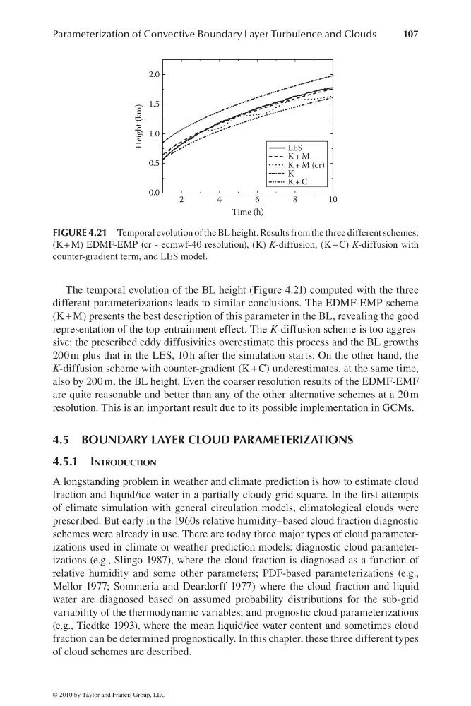
The temporal evolution of the BL height (Figure 4.21) computed with the three
different parameterizations leads to similar conclusions. The EDMF-EMP scheme
(K + M) presents the best description of this parameter in the BL, revealing the good
representation of the top-entrainment effect. The K-diffusion scheme is too aggressive; the prescribed eddy diffusivities overestimate this process and the BL growths
200 m plus that in the LES, 10 h after the simulation starts. On the other hand, the
K-diffusion scheme with counter-gradient (K + C) underestimates, at the same time,
also by 200 m, the BL height. Even the coarser resolution results of the EDMF-EMF
are quite reasonable and better than any of the other alternative schemes at a 20 m
resolution. This is an important result due to its possible implementation in GCMs.
4.5 BOUNDARY LAYER CLOUD PARAMETERIZATIONS
4.5.1 INTRODUCTION
A longstanding problem in weather and climate prediction is how to estimate cloud
fraction and liquid/ice water in a partially cloudy grid square. In the fi rst attempts
of climate simulation with general circulation models, climatological clouds were
prescribed. But early in the 1960s relative humidity–based cloud fraction diagnostic
schemes were already in use. There are today three major types of cloud parameterizations used in climate or weather prediction models: diagnostic cloud parameterizations (e.g., Slingo 1987), where the cloud fraction is diagnosed as a function of
relative humidity and some other parameters; PDF-based parameterizations (e.g.,
Mellor 1977; Sommeria and Deardorff 1977) where the cloud fraction and liquid
water are diagnosed based on assumed probability distributions for the sub-grid
variability of the thermodynamic variables; and prognostic cloud parameterizations
(e.g., Tiedtke 1993), where the mean liquid/ice water content and sometimes cloud
fraction can be determined prognostically. In this chapter, these three different types
of cloud schemes are described.
2.0
1.5
1.0
0.5
0.0
2
4
6
8
1 0
Time (h)
Height (km)
LES
K + M
K + C
K + M (cr)
K
FIGURE 4.21 Temporal evolution of the BL height. Results from the three different schemes:
(K + M) EDMF-EMP (cr - ecmwf-40 resolution), (K) K-diffusion, (K + C) K-diffusion with
counter-gradient term, and LES model.
© 2010 by Taylor and Francis Group, LLC
107
The temporal evolution of the BL height (Figure 4.21) computed with the three
different parameterizations leads to similar conclusions. The EDMF-EMP scheme
(K + M) presents the best description of this parameter in the BL, revealing the good
representation of the top-entrainment effect. The K-diffusion scheme is too aggressive; the prescribed eddy diffusivities overestimate this process and the BL growths
200 m plus that in the LES, 10 h after the simulation starts. On the other hand, the
K-diffusion scheme with counter-gradient (K + C) underestimates, at the same time,
also by 200 m, the BL height. Even the coarser resolution results of the EDMF-EMF
are quite reasonable and better than any of the other alternative schemes at a 20 m
resolution. This is an important result due to its possible implementation in GCMs.
4.5 BOUNDARY LAYER CLOUD PARAMETERIZATIONS
4.5.1 INTRODUCTION
A longstanding problem in weather and climate prediction is how to estimate cloud
fraction and liquid/ice water in a partially cloudy grid square. In the fi rst attempts
of climate simulation with general circulation models, climatological clouds were
prescribed. But early in the 1960s relative humidity–based cloud fraction diagnostic
schemes were already in use. There are today three major types of cloud parameterizations used in climate or weather prediction models: diagnostic cloud parameterizations (e.g., Slingo 1987), where the cloud fraction is diagnosed as a function of
relative humidity and some other parameters; PDF-based parameterizations (e.g.,
Mellor 1977; Sommeria and Deardorff 1977) where the cloud fraction and liquid
water are diagnosed based on assumed probability distributions for the sub-grid
variability of the thermodynamic variables; and prognostic cloud parameterizations
(e.g., Tiedtke 1993), where the mean liquid/ice water content and sometimes cloud
fraction can be determined prognostically. In this chapter, these three different types
of cloud schemes are described.
2.0
1.5
1.0
0.5
0.0
2
4
6
8
1 0
Time (h)
Height (km)
LES
K + M
K + C
K + M (cr)
K
FIGURE 4.21 Temporal evolution of the BL height. Results from the three different schemes:
(K + M) EDMF-EMP (cr - ecmwf-40 resolution), (K) K-diffusion, (K + C) K-diffusion with
counter-gradient term, and LES model.
© 2010 by Taylor and Francis Group, LLC