

Stream Temperature Response to Thermal Pollution
5
T
_ , A a - A e + C a T A | Q s ( K w + KA)
To = T A +
^
+
K W + K A
( 1 0 )
where the overall air heat transfer coefficient is defined as:
K A = B a + Kh + K e
One can obtain an equation describing the heat transfer as:
3t
UL dx
2
3x Hc p p w (K w +K A )
( 1 -
l o j "
U
(11)
Since in turbulent streams, the magnitude of K w is more than two orders of magnitude
greater than KA, the value of K w has little influence on the process of turbulent heat
transfer in streams., and the heat transfer coefficient can be simplified as follows:
K W KA
KA
K = H Cp p w (K w + K A ) ~ H cp p w
APPLICATION OF THE MODEL TO A RIVER TEMPERATURE COMPUTATION
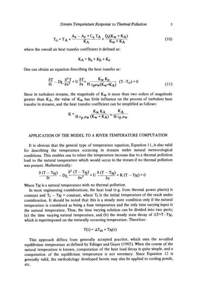
It is obvious that the general type of temperature equation, Equation 11, is also valid
for describing the temperature occurring in streams under natural meteorological
conditions. This enables one to relate the temperature increase due to a thermal pollution
load to the natural temperature which would occur in the stream if no thermal pollution
was present. Mathematically:
3 ( ^ ) ^ 2 ( Τ _ ^ ) ^ 3 _ ( Τ _ Γ ! Ι ) + Κ ( Τ _ Τ Ν ) , Ο
Where TN is a natural temperature with no thermal pollution.
In most engineering considerations, the heat load (e.g. from thermal power plants) is
constant and Tj - T N = constant, where Ti is the initial temperature of the reach under
consideration. It should be noted that this is a steady state condition only if the natural
temperature is considered as being a base temperature and the only time varying input is
the natural temperature. Thus, the time varying solution can be divided into two parts;
(a) the time varying natural temperature, and (b) the steady state decay of Δ Τ = Τ - Τ Ν ,
which is superimposed on the naturally occurring temperature. Therefore:
T(t) = AT ss + T N (t)
This approach differs from generally accepted practice, which uses the so-called
equilibrium temperature as defined by Edinger and Geyer (1965). When the course of the
natural temperature is known, computation of the heat load decay is quite simple, and a
computation of the equilibrium temperature is not necessary. Since Equation 12 is
generally valid, the methodology developed herein may also be applied to cooling ponds,
etc.
5
T
_ , A a - A e + C a T A | Q s ( K w + KA)
To = T A +
^
+
K W + K A
( 1 0 )
where the overall air heat transfer coefficient is defined as:
K A = B a + Kh + K e
One can obtain an equation describing the heat transfer as:
3t
UL dx
2
3x Hc p p w (K w +K A )
( 1 -
l o j "
U
(11)
Since in turbulent streams, the magnitude of K w is more than two orders of magnitude
greater than KA, the value of K w has little influence on the process of turbulent heat
transfer in streams., and the heat transfer coefficient can be simplified as follows:
K W KA
KA
K = H Cp p w (K w + K A ) ~ H cp p w
APPLICATION OF THE MODEL TO A RIVER TEMPERATURE COMPUTATION
It is obvious that the general type of temperature equation, Equation 11, is also valid
for describing the temperature occurring in streams under natural meteorological
conditions. This enables one to relate the temperature increase due to a thermal pollution
load to the natural temperature which would occur in the stream if no thermal pollution
was present. Mathematically:
3 ( ^ ) ^ 2 ( Τ _ ^ ) ^ 3 _ ( Τ _ Γ ! Ι ) + Κ ( Τ _ Τ Ν ) , Ο
Where TN is a natural temperature with no thermal pollution.
In most engineering considerations, the heat load (e.g. from thermal power plants) is
constant and Tj - T N = constant, where Ti is the initial temperature of the reach under
consideration. It should be noted that this is a steady state condition only if the natural
temperature is considered as being a base temperature and the only time varying input is
the natural temperature. Thus, the time varying solution can be divided into two parts;
(a) the time varying natural temperature, and (b) the steady state decay of Δ Τ = Τ - Τ Ν ,
which is superimposed on the naturally occurring temperature. Therefore:
T(t) = AT ss + T N (t)
This approach differs from generally accepted practice, which uses the so-called
equilibrium temperature as defined by Edinger and Geyer (1965). When the course of the
natural temperature is known, computation of the heat load decay is quite simple, and a
computation of the equilibrium temperature is not necessary. Since Equation 12 is
generally valid, the methodology developed herein may also be applied to cooling ponds,
etc.