

et al. (2015b). The error associated with this assumption is particularly
hard to assess using simple back-calculation techniques. Nevertheless,
Touratier et al. (2012) obtained results similar to those of the TrOCA
approach by applying the MIX approach that accounts for the contribution of various water masses in the MS.
3.3.3. Anthropogenic carbon inventory
The estimated metrics and C
ant
inventory for each box are presented
in Table 5. According to our results, the AB sequestered between
0.44 ± 0.06 Pg C (MCM) and 0.53 ± 0.06 Pg C (TrOCA) of C
ant
from
the preindustrial era to the summer of 2014. The magnitude of the
estimated C
ant
inventories is explained by the intrinsic characteristics of
the western MS (high alkalinity, short water renewal times, active
mesoscale structures, etc.) and the increase in atmospheric pCO 2 .
Palmiéri et al. (2015) proposed that the high TA concentrations of the
MS enhance its C
ant
inventory by 10% compared to the global ocean.
Merlivat et al. (2018) indicated that the accumulated DIC during the
last 20 years represents almost 30% of the total inventory of C
ant
in the
MS and that external factors, such as Atlantic inputs, also play an important role in C
ant
sequestration by the MS. According to Palmiéri et al.
(2015), air-sea exchanges alone could explain 75% of the inventory.
The total inventory of C
ant
in the MS was estimated at 1.7 ± 0.4 Pg
C by Schneider et al. (2010) and 1 Pg C by Palmiéri et al. (2015) for
2001. These two inventories were obtained by different techniques
(tracer studies and high resolution model, respectively) and for different spatial and temporal scales. It is thus difficult to compare their
results with those of this study. Nevertheless, as Table 6 illustrates, the
estimated C
ant
inventory of the AB is within the range of those reported
in many other marginal seas in the North Pacific (Chen et al., 2004) and
Atlantic (Jutterström et al., 2008; Olsen et al., 2010) Oceans. The AB is
characterized by higher average excess CO 2 per unit area (1482–1790 g
C.m
−2
) than other marginal seas and oceans because of its intrinsic
properties (like low Revelle Factor): e.g., 400 g C.m
−2
for the Japan Sea
(Park et al., 2006), 800 g C.m
−2
for the Sulu Sea, and 330 g C.m
−2
for
0−150m
150−800m
800−Bottom
0.0 2.5 5.0 7.5 10.0
2 4 8 0
2 5 2 0
2 5 6 0
2 5 7 0
2 5 8 0
2 5 9 0
2 6 0 0
2 6 1 0
2 5 9 0
2 5 9 5
2 6 0 0
2 6 0 5
Longitude
TA (µmol/kg)
(a)
0−150m
150−800m
800−Bottom
0.0 2.5 5.0 7.5 10.0
2 1 5 0
2 2 0 0
2 2 5 0
2 3 0 0
2 3 2 0
2 3 3 0
2 3 4 0
2 3 5 0
2 3 3 0
2 3 3 5
2 3 4 0
2 3 4 5
2 3 5 0
Longitude
DIC (µmol/kg)
(b)
0−150m
150−800m
800−Bottom
0.0 2.5 5.0 7.5 10.0
2 5 4 2 . 5
2 5 4 5 . 0
2 5 4 7 . 5
2 5 5 0 . 0
2 5 5 2 . 5
2 5 5 5 . 0
2 5 4 0
2 5 4 4
2 5 4 8
2 5 4 5
2 5 4 7
2 5 4 9
2 5 5 1
2 5 5 3
Longitude
NTA (µmol/kg)
(c)
0−150m
150−800m
800−Bottom
0.0 2.5 5.0 7.5 10.0
2 2 2 5
2 2 5 0
2 2 7 5
2 3 0 0
2 2 6 0
2 2 6 5
2 2 7 0
2 2 7 5
2 2 8 0
2 2 8 5
2 2 7 4
2 2 7 6
2 2 7 8
2 2 8 0
Longitude
NDIC (µmol/kg)
(d)
0−150m
150−800m
800−Bottom
37
38
39
2 4 5 0
2 5 0 0
2 5 5 0
2 5 6 0
2 5 7 0
2 5 8 0
2 5 9 0
2 6 0 0
2 6 1 0
2 5 8 9
2 5 9 2
2 5 9 5
2 5 9 8
2 6 0 1
Latitude
TA (µmol/kg)
(e)
0−150m
150−800m
800−Bottom
37
38
39
2 1 5 0
2 2 0 0
2 2 5 0
2 3 0 0
2 3 1 0
2 3 2 0
2 3 3 0
2 3 4 0
2 3 5 0
2 3 3 2
2 3 3 6
2 3 4 0
Latitude
DIC (µmol/kg)
(f)
0−150m
150−800m
800−Bottom
37
38
39
2 5 4 5
2 5 5 0
2 5 5 5
2 5 4 0
2 5 4 4
2 5 4 8
2 5 4 4
2 5 4 6
2 5 4 8
2 5 5 0
2 5 5 2
Latitude
NTA (µmol/kg)
(g)
0−150m
150−800m
800−Bottom
37
38
39
2 2 2 5
2 2 5 0
2 2 7 5
2 3 0 0
2 3 2 5
2 2 6 5
2 2 7 0
2 2 7 5
2 2 8 0
2 2 8 5
2 2 7 3
2 2 7 5
2 2 7 7
2 2 7 9
Latitude
NDIC (µmol/kg)
(h)
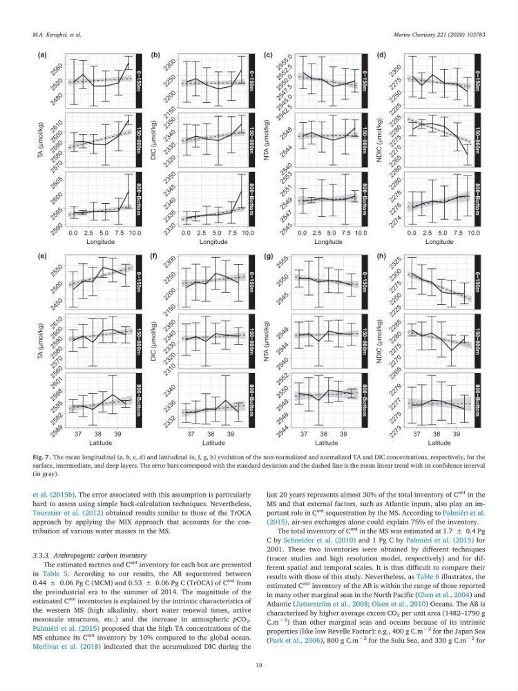
Fig. 7. The mean longitudinal (a, b, c, d) and latitudinal (e, f, g, h) evolution of the non-normalized and normalized TA and DIC concentrations, respectively, for the
surface, intermediate, and deep layers. The error bars correspond with the standard deviation and the dashed line is the mean linear trend with its confidence interval
(in gray).
M.A. Keraghel, et al.
Marine Chemistry 221 (2020) 103783
10
hard to assess using simple back-calculation techniques. Nevertheless,
Touratier et al. (2012) obtained results similar to those of the TrOCA
approach by applying the MIX approach that accounts for the contribution of various water masses in the MS.
3.3.3. Anthropogenic carbon inventory
The estimated metrics and C
ant
inventory for each box are presented
in Table 5. According to our results, the AB sequestered between
0.44 ± 0.06 Pg C (MCM) and 0.53 ± 0.06 Pg C (TrOCA) of C
ant
from
the preindustrial era to the summer of 2014. The magnitude of the
estimated C
ant
inventories is explained by the intrinsic characteristics of
the western MS (high alkalinity, short water renewal times, active
mesoscale structures, etc.) and the increase in atmospheric pCO 2 .
Palmiéri et al. (2015) proposed that the high TA concentrations of the
MS enhance its C
ant
inventory by 10% compared to the global ocean.
Merlivat et al. (2018) indicated that the accumulated DIC during the
last 20 years represents almost 30% of the total inventory of C
ant
in the
MS and that external factors, such as Atlantic inputs, also play an important role in C
ant
sequestration by the MS. According to Palmiéri et al.
(2015), air-sea exchanges alone could explain 75% of the inventory.
The total inventory of C
ant
in the MS was estimated at 1.7 ± 0.4 Pg
C by Schneider et al. (2010) and 1 Pg C by Palmiéri et al. (2015) for
2001. These two inventories were obtained by different techniques
(tracer studies and high resolution model, respectively) and for different spatial and temporal scales. It is thus difficult to compare their
results with those of this study. Nevertheless, as Table 6 illustrates, the
estimated C
ant
inventory of the AB is within the range of those reported
in many other marginal seas in the North Pacific (Chen et al., 2004) and
Atlantic (Jutterström et al., 2008; Olsen et al., 2010) Oceans. The AB is
characterized by higher average excess CO 2 per unit area (1482–1790 g
C.m
−2
) than other marginal seas and oceans because of its intrinsic
properties (like low Revelle Factor): e.g., 400 g C.m
−2
for the Japan Sea
(Park et al., 2006), 800 g C.m
−2
for the Sulu Sea, and 330 g C.m
−2
for
0−150m
150−800m
800−Bottom
0.0 2.5 5.0 7.5 10.0
2 4 8 0
2 5 2 0
2 5 6 0
2 5 7 0
2 5 8 0
2 5 9 0
2 6 0 0
2 6 1 0
2 5 9 0
2 5 9 5
2 6 0 0
2 6 0 5
Longitude
TA (µmol/kg)
(a)
0−150m
150−800m
800−Bottom
0.0 2.5 5.0 7.5 10.0
2 1 5 0
2 2 0 0
2 2 5 0
2 3 0 0
2 3 2 0
2 3 3 0
2 3 4 0
2 3 5 0
2 3 3 0
2 3 3 5
2 3 4 0
2 3 4 5
2 3 5 0
Longitude
DIC (µmol/kg)
(b)
0−150m
150−800m
800−Bottom
0.0 2.5 5.0 7.5 10.0
2 5 4 2 . 5
2 5 4 5 . 0
2 5 4 7 . 5
2 5 5 0 . 0
2 5 5 2 . 5
2 5 5 5 . 0
2 5 4 0
2 5 4 4
2 5 4 8
2 5 4 5
2 5 4 7
2 5 4 9
2 5 5 1
2 5 5 3
Longitude
NTA (µmol/kg)
(c)
0−150m
150−800m
800−Bottom
0.0 2.5 5.0 7.5 10.0
2 2 2 5
2 2 5 0
2 2 7 5
2 3 0 0
2 2 6 0
2 2 6 5
2 2 7 0
2 2 7 5
2 2 8 0
2 2 8 5
2 2 7 4
2 2 7 6
2 2 7 8
2 2 8 0
Longitude
NDIC (µmol/kg)
(d)
0−150m
150−800m
800−Bottom
37
38
39
2 4 5 0
2 5 0 0
2 5 5 0
2 5 6 0
2 5 7 0
2 5 8 0
2 5 9 0
2 6 0 0
2 6 1 0
2 5 8 9
2 5 9 2
2 5 9 5
2 5 9 8
2 6 0 1
Latitude
TA (µmol/kg)
(e)
0−150m
150−800m
800−Bottom
37
38
39
2 1 5 0
2 2 0 0
2 2 5 0
2 3 0 0
2 3 1 0
2 3 2 0
2 3 3 0
2 3 4 0
2 3 5 0
2 3 3 2
2 3 3 6
2 3 4 0
Latitude
DIC (µmol/kg)
(f)
0−150m
150−800m
800−Bottom
37
38
39
2 5 4 5
2 5 5 0
2 5 5 5
2 5 4 0
2 5 4 4
2 5 4 8
2 5 4 4
2 5 4 6
2 5 4 8
2 5 5 0
2 5 5 2
Latitude
NTA (µmol/kg)
(g)
0−150m
150−800m
800−Bottom
37
38
39
2 2 2 5
2 2 5 0
2 2 7 5
2 3 0 0
2 3 2 5
2 2 6 5
2 2 7 0
2 2 7 5
2 2 8 0
2 2 8 5
2 2 7 3
2 2 7 5
2 2 7 7
2 2 7 9
Latitude
NDIC (µmol/kg)
(h)
Fig. 7. The mean longitudinal (a, b, c, d) and latitudinal (e, f, g, h) evolution of the non-normalized and normalized TA and DIC concentrations, respectively, for the
surface, intermediate, and deep layers. The error bars correspond with the standard deviation and the dashed line is the mean linear trend with its confidence interval
(in gray).
M.A. Keraghel, et al.
Marine Chemistry 221 (2020) 103783
10