

Heat Flow and Storage in Soil
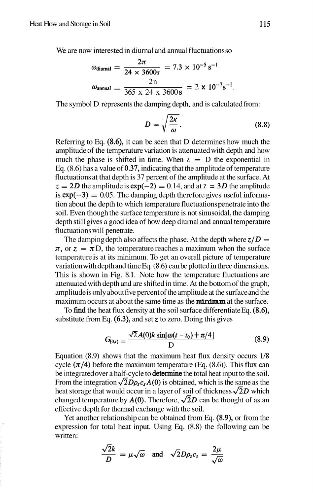
We are now interested in diurnal and annual fluctuations so
2n
wamUal =
= 2 x ~ O - ~ S - ' .
365 x 24 x 3600 s
The symbol D represents the damping depth, and is calculated from:
Referring to Eq. (8.6), it can be seen that D determines how much the
amplitude of the temperature variation is attenuated with depth and how
much the phase is shifted in time. When z = D the exponential in
Eq. (8.6) has a value of 0.37, indicating that the amplitude of temperature
fluctuations at that depth is 37 percent of the amplitude at the surface. At
z = 2 0 the amplitude is exp(-2) = 0.14, and at z = 3 0 the amplitude
is exp(-3) = 0.05. The damping depth therefore gives useful information about the depth to which temperature fluctuations penetrate into the
soil. Even though the surface temperature is not sinusoidal, the damping
depth still gives a good idea of how deep diurnal and annual temperature
fluctuations will penetrate.
The damping depth also affects the phase. At the depth where z/D =
x , or z = x D, the temperature reaches a maximum when the surface
temperature is at its minimum. To get an overall picture of temperature
variation with depth and time Eq. (8.6) can be plotted in three dimensions.
This is shown in Fig. 8.1. Note how the temperature fluctuations are
attenuated with depth and are shifted in time. At the bottom of the graph,
amplitude is only about five percent of the amplitude at the surface and the
maximum occurs at about the same time as the minimum at the surface.
To find the heat flux density at the soil surface differentiate Eq. (8.6),
substitute from Eq. (6.3), and set z to zero. Doing this gives
aA(0)k sin[w(t - to) + n/4]
G(0,t) =
D
(8.9)
Equation (8.9) shows that the maximum heat flux density occurs 118
cycle (n/4) before the maximum temperature (Eq. (8.6)). This flux can
be integrated over a half-cycle to determine the total heat input to the soil.
From the integration fiDpScs~(0) is obtained, which is the same as the
heat storage that would occur in a layer of soil of thickness f i D which
changed temperature by A(0). Therefore, f i D can be thought of as an
effective depth for thermal exchange with the soil.
Yet another relationship can be obtained from Eq. (8.9), or from the
expression for total heat input. Using Eq. (8.8) the following can be
written:
We are now interested in diurnal and annual fluctuations so
2n
wamUal =
= 2 x ~ O - ~ S - ' .
365 x 24 x 3600 s
The symbol D represents the damping depth, and is calculated from:
Referring to Eq. (8.6), it can be seen that D determines how much the
amplitude of the temperature variation is attenuated with depth and how
much the phase is shifted in time. When z = D the exponential in
Eq. (8.6) has a value of 0.37, indicating that the amplitude of temperature
fluctuations at that depth is 37 percent of the amplitude at the surface. At
z = 2 0 the amplitude is exp(-2) = 0.14, and at z = 3 0 the amplitude
is exp(-3) = 0.05. The damping depth therefore gives useful information about the depth to which temperature fluctuations penetrate into the
soil. Even though the surface temperature is not sinusoidal, the damping
depth still gives a good idea of how deep diurnal and annual temperature
fluctuations will penetrate.
The damping depth also affects the phase. At the depth where z/D =
x , or z = x D, the temperature reaches a maximum when the surface
temperature is at its minimum. To get an overall picture of temperature
variation with depth and time Eq. (8.6) can be plotted in three dimensions.
This is shown in Fig. 8.1. Note how the temperature fluctuations are
attenuated with depth and are shifted in time. At the bottom of the graph,
amplitude is only about five percent of the amplitude at the surface and the
maximum occurs at about the same time as the minimum at the surface.
To find the heat flux density at the soil surface differentiate Eq. (8.6),
substitute from Eq. (6.3), and set z to zero. Doing this gives
aA(0)k sin[w(t - to) + n/4]
G(0,t) =
D
(8.9)
Equation (8.9) shows that the maximum heat flux density occurs 118
cycle (n/4) before the maximum temperature (Eq. (8.6)). This flux can
be integrated over a half-cycle to determine the total heat input to the soil.
From the integration fiDpScs~(0) is obtained, which is the same as the
heat storage that would occur in a layer of soil of thickness f i D which
changed temperature by A(0). Therefore, f i D can be thought of as an
effective depth for thermal exchange with the soil.
Yet another relationship can be obtained from Eq. (8.9), or from the
expression for total heat input. Using Eq. (8.8) the following can be
written: