

114
Heat Flow in the Soil
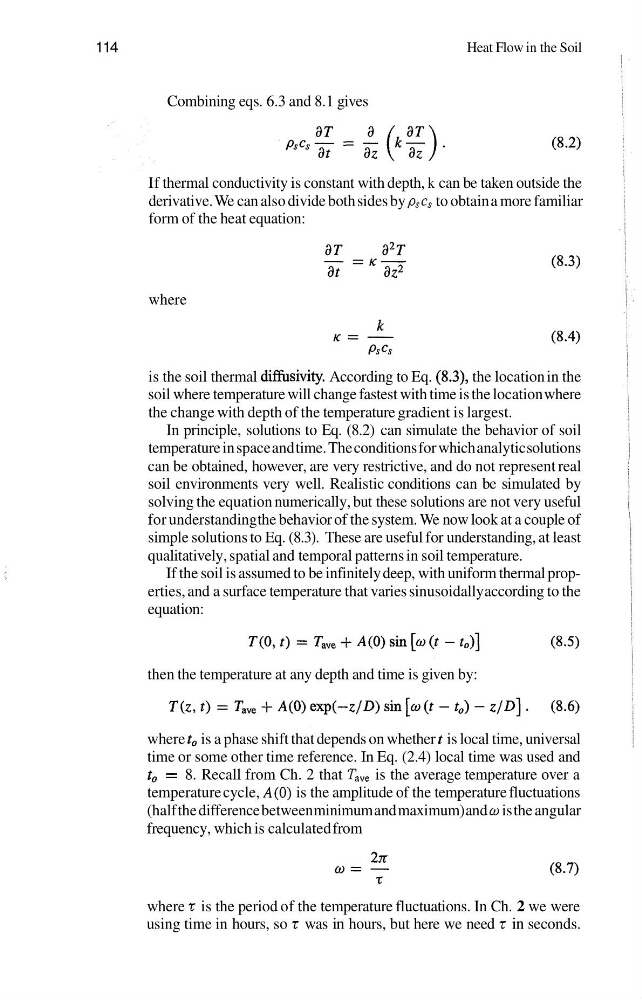
Combining eqs. 6.3 and 8.1 gives
If thermal conductivity is constant with depth, k can be taken outside the
derivative. We can also divide both sides by pscs to obtain a more familiar
form of the heat equation:
where
is the soil thermal diffusivity. According to Eq. (8.3), the location in the
soil where temperature will change fastest with time is the location where
the change with depth of the temperature gradient is largest.
In principle, solutions to Eq. (8.2) can simulate the behavior of soil
temperature in space and time. The conditions for which analytic solutions
can be obtained, however, are very restrictive, and do not represent real
soil environments very well. Realistic conditions can be simulated by
solving the equation numerically, but these solutions are not very useful
for understanding the behavior of the system. We now look at a couple of
simple solutions to Eq. (8.3). These are useful for understanding, at least
qualitatively, spatial and temporal patterns in soil temperature.
If the soil is assumed to be infinitely deep, with uniform thermal properties, and a surface temperature that varies sinusoidally according to the
equation:
then the temperature at any depth and time is given by:
where to is a phase shift that depends on whether t is local time, universal
time or some other time reference. In Eq. (2.4) local time was used and
to = 8. Recall from Ch. 2 that Tave is the average temperature over a
temperature cycle, A(0) is the amplitude of the temperature fluctuations
(half the difference between minimum and maximum) and w is the angular
frequency, which is calculated from
where z is the period of the temperature fluctuations. In Ch. 2 we were
using time in hours, so t was in hours, but here we need t in seconds.
Heat Flow in the Soil
Combining eqs. 6.3 and 8.1 gives
If thermal conductivity is constant with depth, k can be taken outside the
derivative. We can also divide both sides by pscs to obtain a more familiar
form of the heat equation:
where
is the soil thermal diffusivity. According to Eq. (8.3), the location in the
soil where temperature will change fastest with time is the location where
the change with depth of the temperature gradient is largest.
In principle, solutions to Eq. (8.2) can simulate the behavior of soil
temperature in space and time. The conditions for which analytic solutions
can be obtained, however, are very restrictive, and do not represent real
soil environments very well. Realistic conditions can be simulated by
solving the equation numerically, but these solutions are not very useful
for understanding the behavior of the system. We now look at a couple of
simple solutions to Eq. (8.3). These are useful for understanding, at least
qualitatively, spatial and temporal patterns in soil temperature.
If the soil is assumed to be infinitely deep, with uniform thermal properties, and a surface temperature that varies sinusoidally according to the
equation:
then the temperature at any depth and time is given by:
where to is a phase shift that depends on whether t is local time, universal
time or some other time reference. In Eq. (2.4) local time was used and
to = 8. Recall from Ch. 2 that Tave is the average temperature over a
temperature cycle, A(0) is the amplitude of the temperature fluctuations
(half the difference between minimum and maximum) and w is the angular
frequency, which is calculated from
where z is the period of the temperature fluctuations. In Ch. 2 we were
using time in hours, so t was in hours, but here we need t in seconds.