

J-2 Gauss surface normal coordinates: case study ellipsoid-of-revolution 649
Box J.6 (Algorithm for solving the normal equations of the constraint minimum distance mapping).
First forward step. Solve (i), (ii), and (iii) for {x 1 , x 2 , x 3 }:
(i)
x
∧
1 (1 + b
2 x
∧
4 ) = X ⇒ x
∧
1 =
X
1 + b 2 x
∧
4
,
(ii)
x
∧
2 (1 + b
2 x
∧
4 ) = Y ⇒ x
∧
2 =
Y
1 + b 2 x
∧
4
,
(iii)
x
∧
3 (1 + a
2 x
∧
4 ) = Z ⇒ x
∧
3 =
Z
1 + a 2 x
∧
4
.
(J.50)
Second forward step. Substitute {x
∧
1 , x
∧
2 , x
∧
3 , x
∧
4 }:
x
∧2
1 + x
∧2
2 =
1
(1 + b 2 x
∧
4 ) 2
`
X
2 + Y
2 ´
, x
∧2
3 =
1
(1 + a 2 x
∧
4 ) 2 Z
2 ,
b
2 `
x
∧2
1 + x
∧2
2
´
+ a
2 x
∧2
3 − a
2 b
2 ⇔ b
2 X
2 + Y
2
(1 + b 2 x
∧
4 ) 2 + a
2
Z
2
(1 + a 2 x
∧
4 ) 2 − a
2 b
2 = 0 .
(J.51)
The characteristic quadratic equation.
Multiply the rational equation of constraint by (1 + a
2 x 4 )
2 (1 + b
2 x 4 )
2 :
b
2 (1 + a
2 x 4 )
2 `
X
2 + Y
2 ´
+ a
2 (1 + b
2 x 4 )
2 Z
2 − a
2 b
2 (1 + a
2 x 4 )
2 (1 + b
2 x 4 )
2 = 0
⇔
(1 + 2a
2 x 4 + a
4 x
2
4 )b
2 `
X
2 + Y
2 ´
+ (1 + 2b
2 x 4 + b
4 x
2
4 )a
2 Z
2 −
−a
2 b
2 (1 + 2a
2 x 4 + a
4 x
2
4 )(1 + 2b
2 x 4 + b
4 x
2
4 ) = 0 ,
(J.52)
−x
4
4 a
6 b
6 − 2x
3
4 a
4 b
4 (a
2 + b
2 ) + x
2
4 a
2 b
2 [a
2 `
X
2 + Y
2 ´
+ b
2 Z
2 − 4a
2 b
2 − a
4 − b
4 ]+
+2x 4 a
2 b
2 `
X
2 + Y
2 + Z
2 ´
+ b
2 `
X
2 + Y
2 ´
+ a
2 Z
2 − a
2 b
2 = 0 ,
(J.53)
x
4
4 + 2x
3
4
a
2 + b
2
a 2 b 2 + x
2
4
4a
2 b
2 + a
4 + b
4 − a
2
`
X
2 + Y
2
´ − b
2 Z
2
a 4 b 4
−
−2x 4
`
X
2 + Y
2 + Z
2
´
a 4 b 4
−
b
2
`
X
2 + Y
2
´
+ a
2 Z
2 − a
2 b
2
a 6 b 6
= 0 .
(J.54)
Backward step. Substitute {x
∧
1 (x
∧
4 ), x
∧
2 (x
∧
4 ), x
∧
3 (x
∧
4 )}:
x
∧
1 = (1 + b
2 x
∧
4 )
−1 X , x
∧
2 = (1 + b
2 x
∧
4 )
−1 Y , x
∧
3 = (1 + a
2 x
∧
4 )
−1 Z .
(J.55)
Test:
Λ 1 = Λ 2 = 1 + b
2 x
∧
4 > 0, Λ 3 = 1 + a
2 x
∧
4 > 0 if Λ 1 = Λ 2 > 0 and Λ 3 > 0 then end.
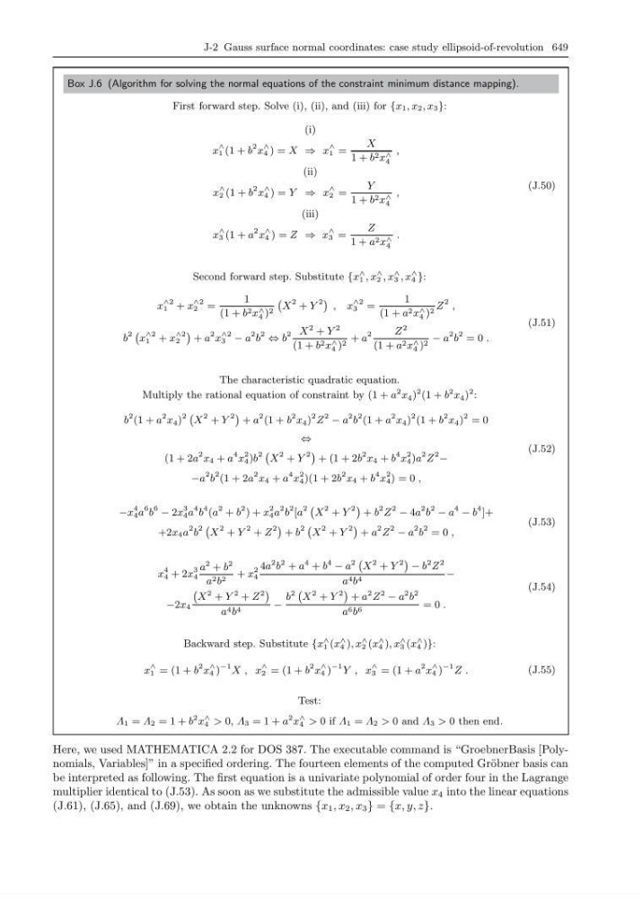
Here, we used MATHEMATICA 2.2 for DOS 387. The executable command is “GroebnerBasis [Polynomials, Variables]” in a specified ordering. The fourteen elements of the computed Gr¨ obner basis can
be interpreted as following. The first equation is a univariate polynomial of order four in the Lagrange
multiplier identical to (J.53). As soon as we substitute the admissible value x 4 into the linear equations
(J.61), (J.65), and (J.69), we obtain the unknowns {x 1 , x 2 , x 3 } = {x, y, z}.