

648 J Gauss surface normal coordinates in geometry and gravity space
Corollary J.4 (E
2
A 1 ,A 2
Gauss differential invariants).
The Gauss differential invariants {I, II, III} of the ellipsoid-of-revolution E
2
A 1 ,A 2
are characterized
by Gauss surface normal coordinates represented by (J.42), (J.43), and (J.44). Especially, the Gauss
map N E
2
A 1 ,A 2
→ S
2 has the spherical metric III.
End of Corollary.
J-22 Buchberger algorithm of forming a constraint minimum distance mapping
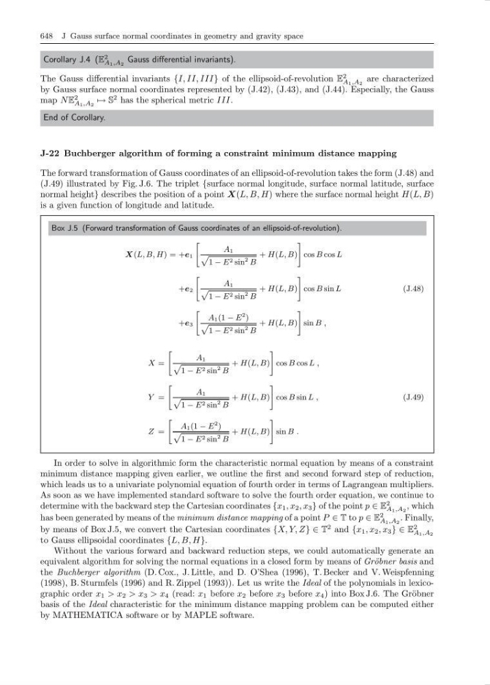
The forward transformation of Gauss coordinates of an ellipsoid-of-revolution takes the form (J.48) and
(J.49) illustrated by Fig. J.6. The triplet {surface normal longitude, surface normal latitude, surface
normal height} describes the position of a point X(L, B, H) where the surface normal height H(L, B)
is a given function of longitude and latitude.
Box J.5 (Forward transformation of Gauss coordinates of an ellipsoid-of-revolution).
X (L, B, H) = +e 1
"
A 1
p
1 − E 2 sin
2 B
+ H(L, B)
#
cos B cos L
+e 2
"
A 1
p
1 − E 2 sin
2 B
+ H(L, B)
#
cos B sin L
+e 3
"
A 1 (1 − E
2 )
p
1 − E 2 sin
2 B
+ H(L, B)
#
sin B ,
(J.48)
X =
"
A 1
p
1 − E 2 sin
2 B
+ H(L, B)
#
cos B cos L ,
Y =
"
A 1
p
1 − E 2 sin
2 B
+ H(L, B)
#
cos B sin L ,
Z =
"
A 1 (1 − E
2 )
p
1 − E 2 sin
2 B
+ H(L, B)
#
sin B .
(J.49)
In order to solve in algorithmic form the characteristic normal equation by means of a constraint
minimum distance mapping given earlier, we outline the first and second forward step of reduction,
which leads us to a univariate polynomial equation of fourth order in terms of Lagrangean multipliers.
As soon as we have implemented standard software to solve the fourth order equation, we continue to
determine with the backward step the Cartesian coordinates {x 1 , x 2 , x 3 } of the point p ∈ E
2
A 1 ,A 2
, which
has been generated by means of the minimum distance mapping of a point P ∈ T to p ∈ E
2
A 1 ,A 2
. Finally,
by means of Box J.5, we convert the Cartesian coordinates {X, Y, Z} ∈ T
2 and {x 1 , x 2 , x 3 } ∈ E
2
A 1 ,A 2
to Gauss ellipsoidal coordinates {L, B, H}.
Without the various forward and backward reduction steps, we could automatically generate an
equivalent algorithm for solving the normal equations in a closed form by means of Gr¨ obner basis and
the Buchberger algorithm (D. Cox., J. Little, and D. O’Shea (1996), T. Becker and V. Weispfenning
(1998), B. Sturmfels (1996) and R. Zippel (1993)). Let us write the Ideal of the polynomials in lexicographic order x 1 > x 2 > x 3 > x 4 (read: x 1 before x 2 before x 3 before x 4 ) into Box J.6. The Gr¨ obner
basis of the Ideal characteristic for the minimum distance mapping problem can be computed either
by MATHEMATICA software or by MAPLE software.