J-2 Gauss surface normal coordinates: case study ellipsoid-of-revolution 647
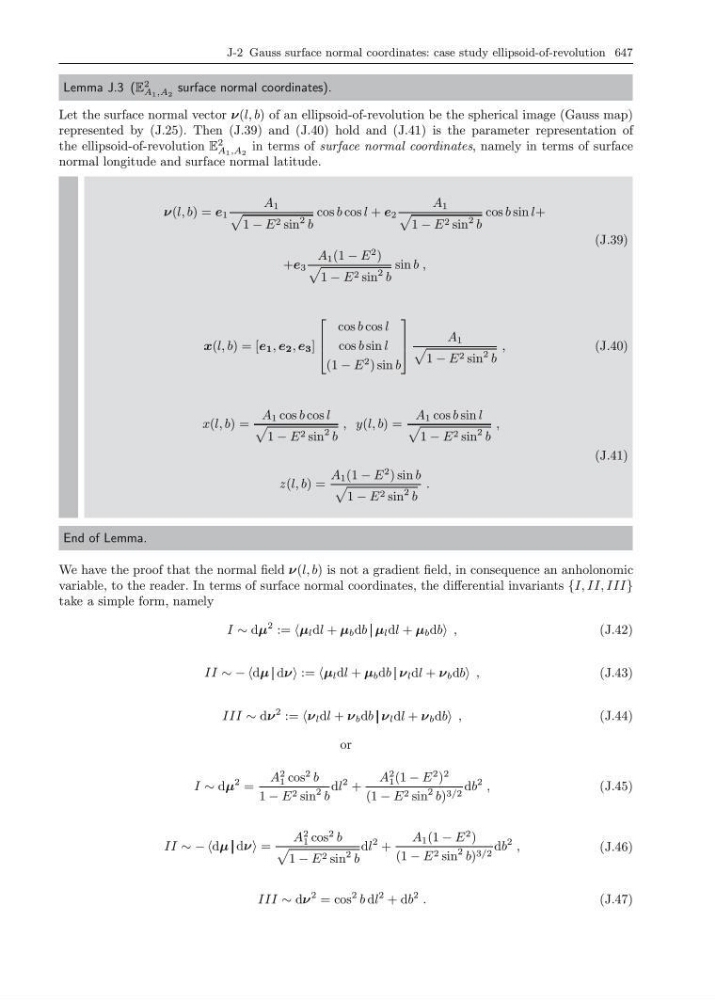
Lemma J.3 (E
2
A 1 ,A 2
surface normal coordinates).
Let the surface normal vector ν(l, b) of an ellipsoid-of-revolution be the spherical image (Gauss map)
represented by (J.25). Then (J.39) and (J.40) hold and (J.41) is the parameter representation of
the ellipsoid-of-revolution E
2
A 1 ,A 2
in terms of surface normal coordinates, namely in terms of surface
normal longitude and surface normal latitude.
ν(l, b) = e 1
A 1
1 − E 2 sin
2 b
cos b cos l + e 2
A 1
1 − E 2 sin
2 b
cos b sin l+
+e 3
A 1 (1 − E
2 )
1 − E 2 sin
2 b
sin b ,
(J.39)
x(l, b) = [e 1 , e 2 , e 3 ]
⎡
⎢
⎣
cos b cos l
cos b sin l
(1 − E
2 ) sin b
⎤
⎥
⎦
A 1
1 − E 2 sin
2 b
,
(J.40)
x(l, b) =
A 1 cos b cos l
1 − E 2 sin
2 b
, y(l, b) =
A 1 cos b sin l
1 − E 2 sin
2 b
,
z(l, b) =
A 1 (1 − E
2 ) sin b
1 − E 2 sin
2 b
.
(J.41)
End of Lemma.
We have the proof that the normal field ν(l, b) is not a gradient field, in consequence an anholonomic
variable, to the reader. In terms of surface normal coordinates, the differential invariants {I, II, III}
take a simple form, namely
I ∼ dµ
2 := µ l dl + µ b db µ l dl + µ b db ,
(J.42)
II ∼ − −dµ dν := µ l dl + µ b db ν l dl + ν b db ,
(J.43)
III ∼ dν
2 := ν l dl + ν b db ν l dl + ν b db ,
(J.44)
or
I ∼ dµ
2 =
A
2
1 cos
2 b
1 − E 2 sin
2 b
dl
2 +
A
2
1 (1 − E
2 )
2
(1 − E 2 sin
2 b) 3/2 db
2 ,
(J.45)
II ∼ − −dµ dν =
A
2
1 cos
2 b
1 − E 2 sin
2 b
dl
2 +
A 1 (1 − E
2 )
(1 − E 2 sin
2 b) 3/2 db
2 ,
(J.46)
III ∼ dν
2 = cos
2 b dl
2 + db
2 .
(J.47)