564 E Geodesics
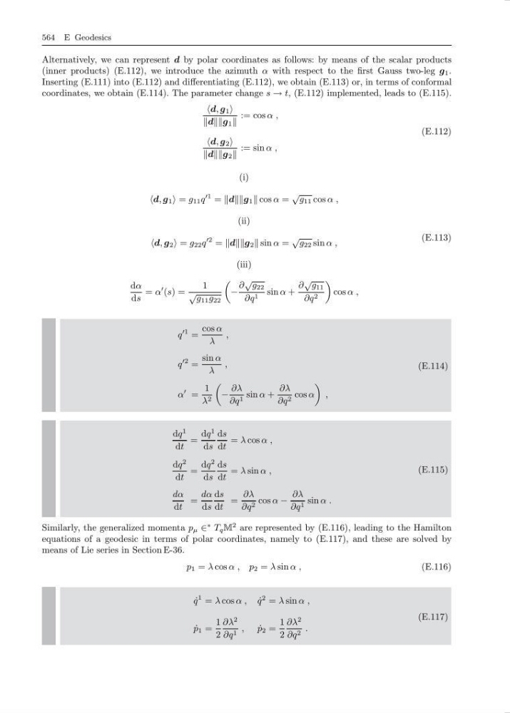
Alternatively, we can represent d by polar coordinates as follows: by means of the scalar products
(inner products) (E.112), we introduce the azimuth α with respect to the first Gauss two-leg g 1 .
Inserting (E.111) into (E.112) and differentiating (E.112), we obtain (E.113) or, in terms of conformal
coordinates, we obtain (E.114). The parameter change s → t, (E.112) implemented, leads to (E.115).
d, g 1
d 1
:= cos α ,
d, g 2
d 2
:= sin α ,
(E.112)
(i)
d, g 1 = g 11 q
1 = d 1 cos α =
√ g 11 cos α ,
(ii)
d, g 2 = g 22 q
2 = d 2 sin α =
√ g 22 sin α ,
(iii)
dα
ds
= α
(s) =
1
√
g 11 g 22
−
∂
√ g 22
∂q 1 sin α +
∂
√
g 11
∂q 2
cos α ,
(E.113)
q
1 =
cos α
λ
,
q
2 =
sin α
λ
,
α
=
1
λ 2
−
∂λ
∂q 1 sin α +
∂λ
∂q 2 cos α
,
(E.114)
dq
1
dt
=
dq
1
ds
ds
dt
= λ cos α ,
dq
2
dt
=
dq
2
ds
ds
dt
= λ sin α ,
dα
dt
=
dα
ds
ds
dt
=
∂λ
∂q 2 cos α −
∂λ
∂q 1 sin α .
(E.115)
Similarly, the generalized momenta p µ ∈
∗ T q M
2 are represented by (E.116), leading to the Hamilton
equations of a geodesic in terms of polar coordinates, namely to (E.117), and these are solved by
means of Lie series in Section E-36.
p 1 = λ cos α , p 2 = λ sin α ,
(E.116)
˙
q
1 = λ cos α , ˙
q
2 = λ sin α ,
˙
p 1 =
1
2
∂λ
2
∂q 1 ,
˙
p 2 =
1
2
∂λ
2
∂q 2 .
(E.117)