

E-3 The Newton form of a geodesic in Maupertuis gauge (sphere, ellipsoid-of-revolution) 565
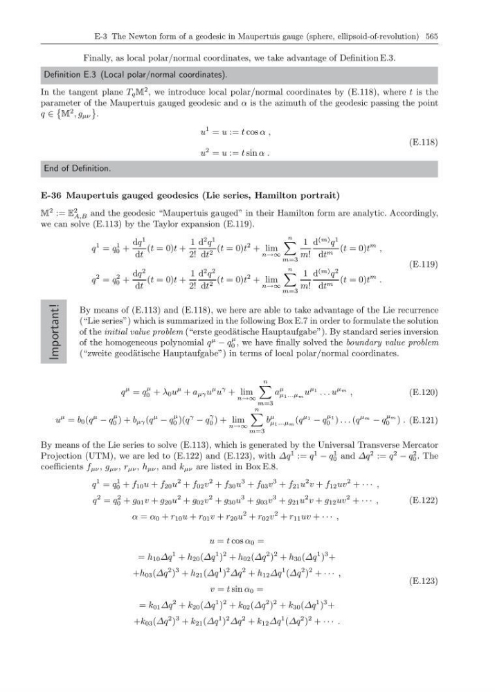
Finally, as local polar/normal coordinates, we take advantage of Definition E.3.
Definition E.3 (Local polar/normal coordinates).
In the tangent plane T q M
2 , we introduce local polar/normal coordinates by (E.118), where t is the
parameter of the Maupertuis gauged geodesic and α is the azimuth of the geodesic passing the point
q ∈
M
2 , g µν
.
u
1 = u := t cos α ,
u
2 = u := t sin α .
(E.118)
End of Definition.
E-36 Maupertuis gauged geodesics (Lie series, Hamilton portrait)
M
2 := E
2
A,B and the geodesic “Maupertuis gauged” in their Hamilton form are analytic. Accordingly,
we can solve (E.113) by the Taylor expansion (E.119).
q
1 = q
1
0 +
dq
1
dt
(t = 0)t +
1
2!
d
2 q
1
dt 2 (t = 0)t
2 + lim
n→∞
n
m=3
1
m!
d
(m) q
1
dt m (t = 0)t
m ,
q
2 = q
2
0 +
dq
2
dt
(t = 0)t +
1
2!
d
2 q
2
dt 2 (t = 0)t
2 + lim
n→∞
n
m=3
1
m!
d
(m) q
2
dt m (t = 0)t
m .
(E.119)
Important!
By means of (E.113) and (E.118), we here are able to take advantage of the Lie recurrence
(“Lie series”) which is summarized in the following Box E.7 in order to formulate the solution
of the initial value problem (“erste geod¨ atische Hauptaufgabe”). By standard series inversion
of the homogeneous polynomial q
µ
− q
µ
0 , we have finally solved the boundary value problem
(“zweite geod¨ atische Hauptaufgabe”) in terms of local polar/normal coordinates.
q
µ = q
µ
0 + λ 0 u
µ + a µγ u
µ u
γ + lim
n→∞
n
m=3
a
µ
µ 1 ...µ m u
µ 1 . . . u
µ m ,
(E.120)
u
µ = b 0 (q
µ
− q
µ
0 ) + b µγ (q
µ
− q
µ
0 )(q
γ
− q
γ
0 ) + lim
n→∞
n
m=3
b
µ
µ 1 ...µ m (q
µ 1 − q
µ 1
0 ) . . . (q
µ m − q
µ m
0 ) . (E.121)
By means of the Lie series to solve (E.113), which is generated by the Universal Transverse Mercator
Projection (UTM), we are led to (E.122) and (E.123), with ∆q
1 := q
1
− q
1
0 and ∆q
2 := q
2
− q
2
0 . The
coefficients f µν , g µν , r µν , h µν , and k µν are listed in Box E.8.
q
1 = q
1
0 + f 10 u + f 20 u
2 + f 02 v
2 + f 30 u
3 + f 03 v
3 + f 21 u
2 v + f 12 uv
2 + · · · ,
q
2 = q
2
0 + g 01 v + g 20 u
2 + g 02 v
2 + g 30 u
3 + g 03 v
3 + g 21 u
2 v + g 12 uv
2 + · · · ,
α = α 0 + r 10 u + r 01 v + r 20 u
2 + r 02 v
2 + r 11 uv + · · · ,
(E.122)
u = t cos α 0 =
= h 10 ∆q
1 + h 20 (∆q
1 )
2 + h 02 (∆q
2 )
2 + h 30 (∆q
1 )
3 +
+h 03 (∆q
2 )
3 + h 21 (∆q
1 )
2 ∆q
2 + h 12 ∆q
1 (∆q
2 )
2 + · · · ,
v = t sin α 0 =
= k 01 ∆q
2 + k 20 (∆q
1 )
2 + k 02 (∆q
2 )
2 + k 30 (∆q
1 )
3 +
+k 03 (∆q
2 )
3 + k 21 (∆q
1 )
2 ∆q
2 + k 12 ∆q
1 (∆q
2 )
2 + · · · .
(E.123)
Finally, as local polar/normal coordinates, we take advantage of Definition E.3.
Definition E.3 (Local polar/normal coordinates).
In the tangent plane T q M
2 , we introduce local polar/normal coordinates by (E.118), where t is the
parameter of the Maupertuis gauged geodesic and α is the azimuth of the geodesic passing the point
q ∈
M
2 , g µν
.
u
1 = u := t cos α ,
u
2 = u := t sin α .
(E.118)
End of Definition.
E-36 Maupertuis gauged geodesics (Lie series, Hamilton portrait)
M
2 := E
2
A,B and the geodesic “Maupertuis gauged” in their Hamilton form are analytic. Accordingly,
we can solve (E.113) by the Taylor expansion (E.119).
q
1 = q
1
0 +
dq
1
dt
(t = 0)t +
1
2!
d
2 q
1
dt 2 (t = 0)t
2 + lim
n→∞
n
m=3
1
m!
d
(m) q
1
dt m (t = 0)t
m ,
q
2 = q
2
0 +
dq
2
dt
(t = 0)t +
1
2!
d
2 q
2
dt 2 (t = 0)t
2 + lim
n→∞
n
m=3
1
m!
d
(m) q
2
dt m (t = 0)t
m .
(E.119)
Important!
By means of (E.113) and (E.118), we here are able to take advantage of the Lie recurrence
(“Lie series”) which is summarized in the following Box E.7 in order to formulate the solution
of the initial value problem (“erste geod¨ atische Hauptaufgabe”). By standard series inversion
of the homogeneous polynomial q
µ
− q
µ
0 , we have finally solved the boundary value problem
(“zweite geod¨ atische Hauptaufgabe”) in terms of local polar/normal coordinates.
q
µ = q
µ
0 + λ 0 u
µ + a µγ u
µ u
γ + lim
n→∞
n
m=3
a
µ
µ 1 ...µ m u
µ 1 . . . u
µ m ,
(E.120)
u
µ = b 0 (q
µ
− q
µ
0 ) + b µγ (q
µ
− q
µ
0 )(q
γ
− q
γ
0 ) + lim
n→∞
n
m=3
b
µ
µ 1 ...µ m (q
µ 1 − q
µ 1
0 ) . . . (q
µ m − q
µ m
0 ) . (E.121)
By means of the Lie series to solve (E.113), which is generated by the Universal Transverse Mercator
Projection (UTM), we are led to (E.122) and (E.123), with ∆q
1 := q
1
− q
1
0 and ∆q
2 := q
2
− q
2
0 . The
coefficients f µν , g µν , r µν , h µν , and k µν are listed in Box E.8.
q
1 = q
1
0 + f 10 u + f 20 u
2 + f 02 v
2 + f 30 u
3 + f 03 v
3 + f 21 u
2 v + f 12 uv
2 + · · · ,
q
2 = q
2
0 + g 01 v + g 20 u
2 + g 02 v
2 + g 30 u
3 + g 03 v
3 + g 21 u
2 v + g 12 uv
2 + · · · ,
α = α 0 + r 10 u + r 01 v + r 20 u
2 + r 02 v
2 + r 11 uv + · · · ,
(E.122)
u = t cos α 0 =
= h 10 ∆q
1 + h 20 (∆q
1 )
2 + h 02 (∆q
2 )
2 + h 30 (∆q
1 )
3 +
+h 03 (∆q
2 )
3 + h 21 (∆q
1 )
2 ∆q
2 + h 12 ∆q
1 (∆q
2 )
2 + · · · ,
v = t sin α 0 =
= k 01 ∆q
2 + k 20 (∆q
1 )
2 + k 02 (∆q
2 )
2 + k 30 (∆q
1 )
3 +
+k 03 (∆q
2 )
3 + k 21 (∆q
1 )
2 ∆q
2 + k 12 ∆q
1 (∆q
2 )
2 + · · · .
(E.123)