

E-3 The Newton form of a geodesic in Maupertuis gauge (sphere, ellipsoid-of-revolution) 549
dq
µ
dτ
=
∂H
2
∂p µ
= g
µν p ν ∀ g
µν =
1
λ 2 (q 1 , q 2 )
δ µν ,
dp µ
dτ
= −
∂H
2
∂q µ = −
1
2
∂g
αβ
∂q µ p α p β ∀ g
µν =
1
λ 2 (q 1 , q 2 )
δ µν ,
(E.26)
dq
µ
dτ
=
∂H
2
∂p µ
=
1
λ 2 (q 1 , q 2 )
p µ ,
dp µ
dτ
= −
(p
2
1 + p
2
2 )
2
∂
∂q µ
1
λ 2 (q 1 , q 2 )
.
(E.27)
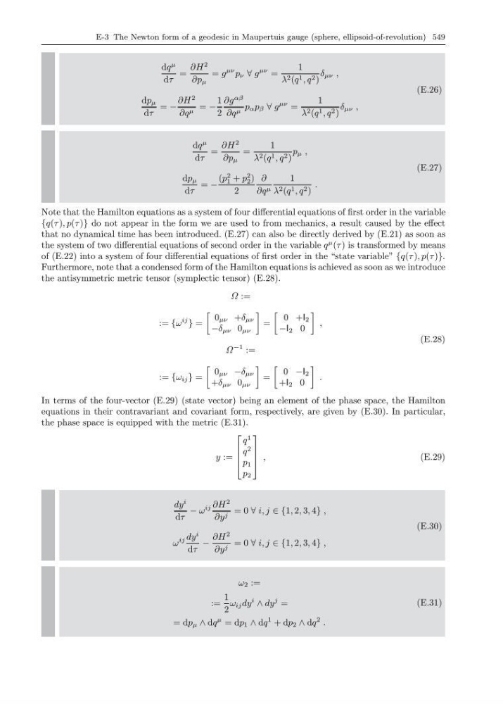
Note that the Hamilton equations as a system of four differential equations of first order in the variable
{q(τ ), p(τ )} do not appear in the form we are used to from mechanics, a result caused by the effect
that no dynamical time has been introduced. (E.27) can also be directly derived by (E.21) as soon as
the system of two differential equations of second order in the variable q
µ (τ ) is transformed by means
of (E.22) into a system of four differential equations of first order in the “state variable” {q(τ ), p(τ )}.
Furthermore, note that a condensed form of the Hamilton equations is achieved as soon as we introduce
the antisymmetric metric tensor (symplectic tensor) (E.28).
Ω :=
:= {ω
ij
} =
0 µν +δ µν
−δ µν 0 µν
=
0 +I 2
−I 2 0
,
Ω
−1 :=
:= {ω ij } =
0 µν −δ µν
+δ µν 0 µν
=
0 −I 2
+I 2 0
.
(E.28)
In terms of the four-vector (E.29) (state vector) being an element of the phase space, the Hamilton
equations in their contravariant and covariant form, respectively, are given by (E.30). In particular,
the phase space is equipped with the metric (E.31).
y :=
⎡
⎢
⎢
⎣
q
1
q
2
p 1
p 2
⎤
⎥
⎥
⎦ ,
(E.29)
dy
i
dτ
− ω
ij ∂H
2
∂y j = 0 ∀ i, j ∈ {1, 2, 3, 4} ,
ω
ij dy
i
dτ
−
∂H
2
∂y j = 0 ∀ i, j ∈ {1, 2, 3, 4} ,
(E.30)
ω 2 :=
:=
1
2
ω ij dy
i
∧ dy
j =
= dp µ ∧ dq
µ = dp 1 ∧ dq
1 + dp 2 ∧ dq
2 .
(E.31)
dq
µ
dτ
=
∂H
2
∂p µ
= g
µν p ν ∀ g
µν =
1
λ 2 (q 1 , q 2 )
δ µν ,
dp µ
dτ
= −
∂H
2
∂q µ = −
1
2
∂g
αβ
∂q µ p α p β ∀ g
µν =
1
λ 2 (q 1 , q 2 )
δ µν ,
(E.26)
dq
µ
dτ
=
∂H
2
∂p µ
=
1
λ 2 (q 1 , q 2 )
p µ ,
dp µ
dτ
= −
(p
2
1 + p
2
2 )
2
∂
∂q µ
1
λ 2 (q 1 , q 2 )
.
(E.27)
Note that the Hamilton equations as a system of four differential equations of first order in the variable
{q(τ ), p(τ )} do not appear in the form we are used to from mechanics, a result caused by the effect
that no dynamical time has been introduced. (E.27) can also be directly derived by (E.21) as soon as
the system of two differential equations of second order in the variable q
µ (τ ) is transformed by means
of (E.22) into a system of four differential equations of first order in the “state variable” {q(τ ), p(τ )}.
Furthermore, note that a condensed form of the Hamilton equations is achieved as soon as we introduce
the antisymmetric metric tensor (symplectic tensor) (E.28).
Ω :=
:= {ω
ij
} =
0 µν +δ µν
−δ µν 0 µν
=
0 +I 2
−I 2 0
,
Ω
−1 :=
:= {ω ij } =
0 µν −δ µν
+δ µν 0 µν
=
0 −I 2
+I 2 0
.
(E.28)
In terms of the four-vector (E.29) (state vector) being an element of the phase space, the Hamilton
equations in their contravariant and covariant form, respectively, are given by (E.30). In particular,
the phase space is equipped with the metric (E.31).
y :=
⎡
⎢
⎢
⎣
q
1
q
2
p 1
p 2
⎤
⎥
⎥
⎦ ,
(E.29)
dy
i
dτ
− ω
ij ∂H
2
∂y j = 0 ∀ i, j ∈ {1, 2, 3, 4} ,
ω
ij dy
i
dτ
−
∂H
2
∂y j = 0 ∀ i, j ∈ {1, 2, 3, 4} ,
(E.30)
ω 2 :=
:=
1
2
ω ij dy
i
∧ dy
j =
= dp µ ∧ dq
µ = dp 1 ∧ dq
1 + dp 2 ∧ dq
2 .
(E.31)