

550 E Geodesics
E-32 The Maupertuis gauge and the Newton portrait of a geodesic
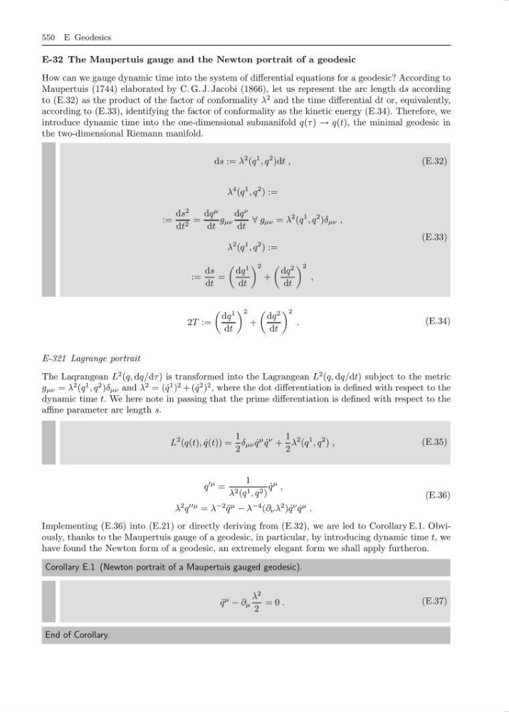
How can we gauge dynamic time into the system of differential equations for a geodesic? According to
Maupertuis (1744) elaborated by C. G. J. Jacobi (1866), let us represent the arc length ds according
to (E.32) as the product of the factor of conformality λ
2 and the time differential dt or, equivalently,
according to (E.33), identifying the factor of conformality as the kinetic energy (E.34). Therefore, we
introduce dynamic time into the one-dimensional submanifold q(τ ) → q(t), the minimal geodesic in
the two-dimensional Riemann manifold.
ds := λ
2 (q
1 , q
2 )dt ,
(E.32)
λ
4 (q
1 , q
2 ) :=
:=
ds
2
dt 2 =
dq
µ
dt
g µν
dq
ν
dt
∀ g µν = λ
2 (q
1 , q
2 )δ µν ,
λ
2 (q
1 , q
2 ) :=
:=
ds
dt
=
dq
1
dt
2
+
dq
2
dt
2
,
(E.33)
2T :=
dq
1
dt
2
+
dq
2
dt
2
.
(E.34)
E-321 Lagrange portrait
The Laqrangean L
2 (q, dq/dτ ) is transformed into the Lagrangean L
2 (q, dq/dt) subject to the metric
g µν = λ
2 (q
1 , q
2 )δ µν and λ
2 = ( ˙
q
1 )
2 + ( ˙
q
2 )
2 , where the dot differentiation is defined with respect to the
dynamic time t. We here note in passing that the prime differentiation is defined with respect to the
affine parameter arc length s.
L
2 (q(t), ˙
q(t)) =
1
2
δ µν ˙
q
µ ˙
q
ν +
1
2
λ
2 (q
1 , q
2 ) ,
(E.35)
q
µ =
1
λ 2 (q 1 , q 2 )
˙
q
µ ,
λ
2 q
= λ
−2 ¨
q
µ
− λ
−4 (∂ ν λ
2 ) ˙
q
ν ˙
q
µ .
(E.36)
Implementing (E.36) into (E.21) or directly deriving from (E.32), we are led to Corollary E.1. Obviously, thanks to the Maupertuis gauge of a geodesic, in particular, by introducing dynamic time t, we
have found the Newton form of a geodesic, an extremely elegant form we shall apply furtheron.
Corollary E.1 (Newton portrait of a Maupertuis gauged geodesic).
¨
q
µ
− ∂ µ
λ
2
2
= 0 .
(E.37)
End of Corollary.
E-32 The Maupertuis gauge and the Newton portrait of a geodesic
How can we gauge dynamic time into the system of differential equations for a geodesic? According to
Maupertuis (1744) elaborated by C. G. J. Jacobi (1866), let us represent the arc length ds according
to (E.32) as the product of the factor of conformality λ
2 and the time differential dt or, equivalently,
according to (E.33), identifying the factor of conformality as the kinetic energy (E.34). Therefore, we
introduce dynamic time into the one-dimensional submanifold q(τ ) → q(t), the minimal geodesic in
the two-dimensional Riemann manifold.
ds := λ
2 (q
1 , q
2 )dt ,
(E.32)
λ
4 (q
1 , q
2 ) :=
:=
ds
2
dt 2 =
dq
µ
dt
g µν
dq
ν
dt
∀ g µν = λ
2 (q
1 , q
2 )δ µν ,
λ
2 (q
1 , q
2 ) :=
:=
ds
dt
=
dq
1
dt
2
+
dq
2
dt
2
,
(E.33)
2T :=
dq
1
dt
2
+
dq
2
dt
2
.
(E.34)
E-321 Lagrange portrait
The Laqrangean L
2 (q, dq/dτ ) is transformed into the Lagrangean L
2 (q, dq/dt) subject to the metric
g µν = λ
2 (q
1 , q
2 )δ µν and λ
2 = ( ˙
q
1 )
2 + ( ˙
q
2 )
2 , where the dot differentiation is defined with respect to the
dynamic time t. We here note in passing that the prime differentiation is defined with respect to the
affine parameter arc length s.
L
2 (q(t), ˙
q(t)) =
1
2
δ µν ˙
q
µ ˙
q
ν +
1
2
λ
2 (q
1 , q
2 ) ,
(E.35)
q
µ =
1
λ 2 (q 1 , q 2 )
˙
q
µ ,
λ
2 q
= λ
−2 ¨
q
µ
− λ
−4 (∂ ν λ
2 ) ˙
q
ν ˙
q
µ .
(E.36)
Implementing (E.36) into (E.21) or directly deriving from (E.32), we are led to Corollary E.1. Obviously, thanks to the Maupertuis gauge of a geodesic, in particular, by introducing dynamic time t, we
have found the Newton form of a geodesic, an extremely elegant form we shall apply furtheron.
Corollary E.1 (Newton portrait of a Maupertuis gauged geodesic).
¨
q
µ
− ∂ µ
λ
2
2
= 0 .
(E.37)
End of Corollary.