

538 D Korn–Lichtenstein and d’Alembert–Euler equations
Solution of the boundary value problem.
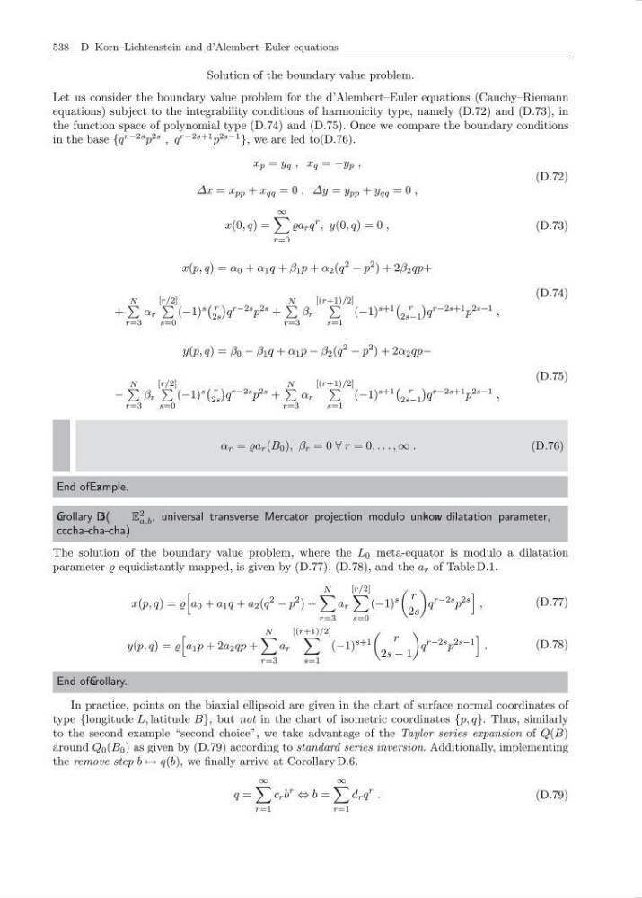
Let us consider the boundary value problem for the d’Alembert–Euler equations (Cauchy–Riemann
equations) subject to the integrability conditions of harmonicity type, namely (D.72) and (D.73), in
the function space of polynomial type (D.74) and (D.75). Once we compare the boundary conditions
in the base {q
r−2s p
2s , q
r−2s+1 p
2s−1
}, we are led to(D.76).
x p = y q , x q = −y p ,
∆x = x pp + x qq = 0 , ∆y = y pp + y qq = 0 ,
(D.72)
x(0, q) =
∞
r=0
r q
r , y(0, q) = 0 ,
(D.73)
x(p, q) = α 0 + α 1 q + β 1 p + α 2 (q
2
− p
2 ) + 2β 2 qp+
+
N
r=3
α r
[r/2]
s=0
(−1)
s
r
2s
q
r−2s p
2s +
N
r=3
β r
[(r+1)/2]
s=1
(−1)
s+1
r
2s−1
q
r−2s+1 p
2s−1 ,
(D.74)
y(p, q) = β 0 − β 1 q + α 1 p − β 2 (q
2
− p
2 ) + 2α 2 qp−
−
N
r=3
β r
[r/2]
s=0
(−1)
s
r
2s
q
r−2s p
2s +
N
r=3
α r
[(r+1)/2]
s=1
(−1)
s+1
r
2s−1
q
r−2s+1 p
2s−1 ,
(D.75)
α r = r (B 0 ), β r = 0 ∀ r = 0, . . . , ∞ .
(D.76)
End ofEx ample.
C
orollary D
.5(
E
2
a,b , universal transverse Mercator projection modulo unk now n dilatation parameter,
c: c: cha–cha–cha) .
The solution of the boundary value problem, where the L 0 meta-equator is modulo a dilatation
parameter equidistantly mapped, is given by (D.77), (D.78), and the a r of Table D.1.
x(p, q) =
a 0 + a 1 q + a 2 (q
2
− p
2 ) +
N
r=3
a r
[r/2]
s=0
(−1)
s
r
2s
q
r−2s p
2s
,
(D.77)
y(p, q) =
a 1 p + 2a 2 qp +
N
r=3
a r
[(r+1)/2]
s=1
(−1)
s+1
r
2s − 1
q
r−2s p
2s−1
.
(D.78)
End ofC orollary.
In practice, points on the biaxial ellipsoid are given in the chart of surface normal coordinates of
type {longitude L, latitude B}, but not in the chart of isometric coordinates {p, q}. Thus, similarly
to the second example “second choice”, we take advantage of the Taylor series expansion of Q(B)
around Q 0 (B 0 ) as given by (D.79) according to standard series inversion. Additionally, implementing
the remove step b → q(b), we finally arrive at Corollary D.6.
q =
∞
r=1
c r b
r
⇔ b =
∞
r=1
d r q
r .
(D.79)
Solution of the boundary value problem.
Let us consider the boundary value problem for the d’Alembert–Euler equations (Cauchy–Riemann
equations) subject to the integrability conditions of harmonicity type, namely (D.72) and (D.73), in
the function space of polynomial type (D.74) and (D.75). Once we compare the boundary conditions
in the base {q
r−2s p
2s , q
r−2s+1 p
2s−1
}, we are led to(D.76).
x p = y q , x q = −y p ,
∆x = x pp + x qq = 0 , ∆y = y pp + y qq = 0 ,
(D.72)
x(0, q) =
∞
r=0
r q
r , y(0, q) = 0 ,
(D.73)
x(p, q) = α 0 + α 1 q + β 1 p + α 2 (q
2
− p
2 ) + 2β 2 qp+
+
N
r=3
α r
[r/2]
s=0
(−1)
s
r
2s
q
r−2s p
2s +
N
r=3
β r
[(r+1)/2]
s=1
(−1)
s+1
r
2s−1
q
r−2s+1 p
2s−1 ,
(D.74)
y(p, q) = β 0 − β 1 q + α 1 p − β 2 (q
2
− p
2 ) + 2α 2 qp−
−
N
r=3
β r
[r/2]
s=0
(−1)
s
r
2s
q
r−2s p
2s +
N
r=3
α r
[(r+1)/2]
s=1
(−1)
s+1
r
2s−1
q
r−2s+1 p
2s−1 ,
(D.75)
α r = r (B 0 ), β r = 0 ∀ r = 0, . . . , ∞ .
(D.76)
End ofEx ample.
C
orollary D
.5(
E
2
a,b , universal transverse Mercator projection modulo unk now n dilatation parameter,
c: c: cha–cha–cha) .
The solution of the boundary value problem, where the L 0 meta-equator is modulo a dilatation
parameter equidistantly mapped, is given by (D.77), (D.78), and the a r of Table D.1.
x(p, q) =
a 0 + a 1 q + a 2 (q
2
− p
2 ) +
N
r=3
a r
[r/2]
s=0
(−1)
s
r
2s
q
r−2s p
2s
,
(D.77)
y(p, q) =
a 1 p + 2a 2 qp +
N
r=3
a r
[(r+1)/2]
s=1
(−1)
s+1
r
2s − 1
q
r−2s p
2s−1
.
(D.78)
End ofC orollary.
In practice, points on the biaxial ellipsoid are given in the chart of surface normal coordinates of
type {longitude L, latitude B}, but not in the chart of isometric coordinates {p, q}. Thus, similarly
to the second example “second choice”, we take advantage of the Taylor series expansion of Q(B)
around Q 0 (B 0 ) as given by (D.79) according to standard series inversion. Additionally, implementing
the remove step b → q(b), we finally arrive at Corollary D.6.
q =
∞
r=1
c r b
r
⇔ b =
∞
r=1
d r q
r .
(D.79)