

536 D Korn–Lichtenstein and d’Alembert–Euler equations
Example D.2 (S
2
r , transverse Mercator projection).
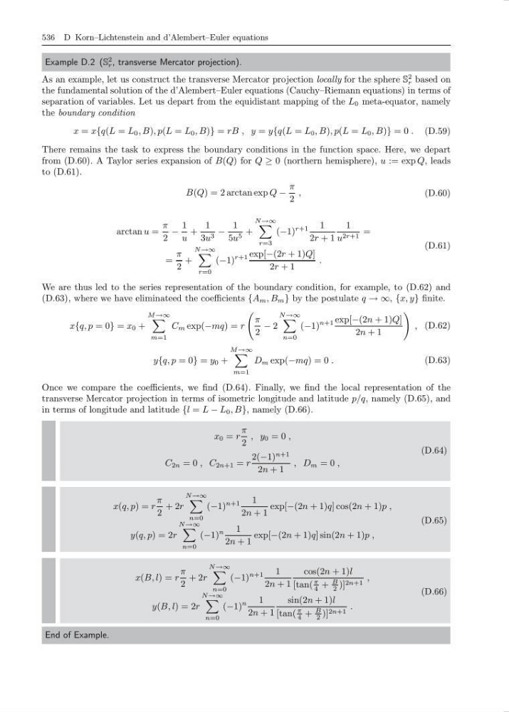
As an example, let us construct the transverse Mercator projection locally for the sphere S
2
r based on
the fundamental solution of the d’Alembert–Euler equations (Cauchy–Riemann equations) in terms of
separation of variables. Let us depart from the equidistant mapping of the L 0 meta-equator, namely
the boundary condition
x = x{q(L = L 0 , B), p(L = L 0 , B)} = rB , y = y{q(L = L 0 , B), p(L = L 0 , B)} = 0 . (D.59)
There remains the task to express the boundary conditions in the function space. Here, we depart
from (D.60). A Taylor series expansion of B(Q) for Q ≥ 0 (northern hemisphere), u := exp Q, leads
to (D.61).
B(Q) = 2 arctan exp Q −
π
2
,
(D.60)
arctan u =
π
2
−
1
u
+
1
3u 3 −
1
5u 5 +
N →∞
r=3
(−1)
r+1
1
2r + 1
1
u 2r+1 =
=
π
2
+
N →∞
r=0
(−1)
r+1 exp[−(2r + 1)Q]
2r + 1
.
(D.61)
We are thus led to the series representation of the boundary condition, for example, to (D.62) and
(D.63), where we have eliminateed the coefficients {A m , B m } by the postulate q → ∞, {x, y} finite.
x{q, p = 0} = x 0 +
M →∞
m=1
C m exp(−mq) = r
π
2
− 2
N →∞
n=0
(−1)
n+1 exp[−(2n + 1)Q]
2n + 1
, (D.62)
y{q, p = 0} = y 0 +
M →∞
m=1
D m exp(−mq) = 0 .
(D.63)
Once we compare the coefficients, we find (D.64). Finally, we find the local representation of the
transverse Mercator projection in terms of isometric longitude and latitude p/q, namely (D.65), and
in terms of longitude and latitude {l = L − L 0 , B}, namely (D.66).
x 0 = r
π
2
, y 0 = 0 ,
C 2n = 0 , C 2n+1 = r
2(−1)
n+1
2n + 1
, D m = 0 ,
(D.64)
x(q, p) = r
π
2
+ 2r
N →∞
n=0
(−1)
n+1
1
2n + 1
exp[−(2n + 1)q] cos(2n + 1)p ,
y(q, p) = 2r
N →∞
n=0
(−1)
n
1
2n + 1
exp[−(2n + 1)q] sin(2n + 1)p ,
(D.65)
x(B, l) = r
π
2
+ 2r
N →∞
n=0
(−1)
n+1
1
2n + 1
cos(2n + 1)l
[tan(
π
4 +
B
2 )] 2n+1 ,
y(B, l) = 2r
N →∞
n=0
(−1)
n
1
2n + 1
sin(2n + 1)l
[tan(
π
4 +
B
2 )] 2n+1 .
(D.66)
End of Example.
Example D.2 (S
2
r , transverse Mercator projection).
As an example, let us construct the transverse Mercator projection locally for the sphere S
2
r based on
the fundamental solution of the d’Alembert–Euler equations (Cauchy–Riemann equations) in terms of
separation of variables. Let us depart from the equidistant mapping of the L 0 meta-equator, namely
the boundary condition
x = x{q(L = L 0 , B), p(L = L 0 , B)} = rB , y = y{q(L = L 0 , B), p(L = L 0 , B)} = 0 . (D.59)
There remains the task to express the boundary conditions in the function space. Here, we depart
from (D.60). A Taylor series expansion of B(Q) for Q ≥ 0 (northern hemisphere), u := exp Q, leads
to (D.61).
B(Q) = 2 arctan exp Q −
π
2
,
(D.60)
arctan u =
π
2
−
1
u
+
1
3u 3 −
1
5u 5 +
N →∞
r=3
(−1)
r+1
1
2r + 1
1
u 2r+1 =
=
π
2
+
N →∞
r=0
(−1)
r+1 exp[−(2r + 1)Q]
2r + 1
.
(D.61)
We are thus led to the series representation of the boundary condition, for example, to (D.62) and
(D.63), where we have eliminateed the coefficients {A m , B m } by the postulate q → ∞, {x, y} finite.
x{q, p = 0} = x 0 +
M →∞
m=1
C m exp(−mq) = r
π
2
− 2
N →∞
n=0
(−1)
n+1 exp[−(2n + 1)Q]
2n + 1
, (D.62)
y{q, p = 0} = y 0 +
M →∞
m=1
D m exp(−mq) = 0 .
(D.63)
Once we compare the coefficients, we find (D.64). Finally, we find the local representation of the
transverse Mercator projection in terms of isometric longitude and latitude p/q, namely (D.65), and
in terms of longitude and latitude {l = L − L 0 , B}, namely (D.66).
x 0 = r
π
2
, y 0 = 0 ,
C 2n = 0 , C 2n+1 = r
2(−1)
n+1
2n + 1
, D m = 0 ,
(D.64)
x(q, p) = r
π
2
+ 2r
N →∞
n=0
(−1)
n+1
1
2n + 1
exp[−(2n + 1)q] cos(2n + 1)p ,
y(q, p) = 2r
N →∞
n=0
(−1)
n
1
2n + 1
exp[−(2n + 1)q] sin(2n + 1)p ,
(D.65)
x(B, l) = r
π
2
+ 2r
N →∞
n=0
(−1)
n+1
1
2n + 1
cos(2n + 1)l
[tan(
π
4 +
B
2 )] 2n+1 ,
y(B, l) = 2r
N →∞
n=0
(−1)
n
1
2n + 1
sin(2n + 1)l
[tan(
π
4 +
B
2 )] 2n+1 .
(D.66)
End of Example.