

D-2 D’Alembert–Euler (Cauchy–Riemann) equations 535
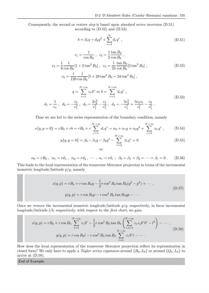
Consequently, the second or restore step is based upon standard series inversion (D.51)
according to (D.52) and (D.53).
b = d 1 q + d 2 q
2 +
∞
r=3
d r q
r ,
(D.51)
c 1 =
1
cos B 0
, c 2 =
1
2
tan B 0
cos B 0
,
c 3 =
1
6
1
cos B 0
[1 + 2 tan
2 B 0 ] , c 4 =
1
24
tan B 0
cos B 0
[5 tan
2 B 0 ] ,
c 5 =
1
120
1
cos B 0
[5 + 28 tan
2 B 0 + 24 tan
4 B 0 ] ,
(D.52)
q =
N →∞
r=1
c r b
r
⇔ b =
N →∞
r=1
d r q
r ,
d 1 =
1
c 1
, d 2 = −
c 2
c 3
1
, d 3 =
2c
2
2
c 5
1
−
c 3
c 4
1
, d 4 = −
5c
3
2
c 7
1
+
5c 2 c 3
c 5
1
−
c 4
c 5
1
.
(D.53)
Thus we are led to the series representation of the boundary condition, namely
x{q, p = 0} = rB 0 + rb = rB 0 + r
N →∞
r=1
d r q
r = α 0 + α 1 q + α 2 q
2 +
N →∞
r=3
α r q
r ,
(D.54)
y{q, p = 0} = β 0 − β 1 q − β 2 q
2
−
N →∞
r=3
β r q
r = 0
(D.55)
⇔
α 0 = rB 0 , α 1 = rd 1 , α 2 = rd 2 , · · · , α r = rd r ; β 0 = β 1 = β 2 = · · · = β r = 0 .
(D.56)
This leads to the local representation of the transverse Mercator projection in terms of the incremental
isometric longitude/latitude p/q, namely
x(q, p) = rB 0 + r cos B 0 q −
1
2
r cos
2 B 0 tan B 0 (q
2
− p
2 ) + · · · ,
y(q, p) = r cos B 0 p − r cos
2 B 0 tan B 0 qp − · · · .
(D.57)
Once we remove the incremental isometric longitude/latitude p/q, respectively, in favor incremental
longitude/latitude l/b, respectively, with respect to the first chart, we gain
x(q, p) = rB 0 + r cos B 0
N →∞
r=1
c r b
r
−
1
2
r cos
2 B 0 tan B 0
N →∞
r,s=1
c r c s b
r b
s
− l
2
− · · · ,
y(q, p) = r cos B 0 l − r cos
2 B 0 tan B 0
N →∞
r=1
c r b
r l − · · · .
(D.58)
How does the local representation of the transverse Mercator projection reflect its representation in
closed form? We only have to apply a Taylor series expansion around {B 0 , L 0 } or around {Q 0 , L 0 } to
arrive at (D.58).
End of Example.
Consequently, the second or restore step is based upon standard series inversion (D.51)
according to (D.52) and (D.53).
b = d 1 q + d 2 q
2 +
∞
r=3
d r q
r ,
(D.51)
c 1 =
1
cos B 0
, c 2 =
1
2
tan B 0
cos B 0
,
c 3 =
1
6
1
cos B 0
[1 + 2 tan
2 B 0 ] , c 4 =
1
24
tan B 0
cos B 0
[5 tan
2 B 0 ] ,
c 5 =
1
120
1
cos B 0
[5 + 28 tan
2 B 0 + 24 tan
4 B 0 ] ,
(D.52)
q =
N →∞
r=1
c r b
r
⇔ b =
N →∞
r=1
d r q
r ,
d 1 =
1
c 1
, d 2 = −
c 2
c 3
1
, d 3 =
2c
2
2
c 5
1
−
c 3
c 4
1
, d 4 = −
5c
3
2
c 7
1
+
5c 2 c 3
c 5
1
−
c 4
c 5
1
.
(D.53)
Thus we are led to the series representation of the boundary condition, namely
x{q, p = 0} = rB 0 + rb = rB 0 + r
N →∞
r=1
d r q
r = α 0 + α 1 q + α 2 q
2 +
N →∞
r=3
α r q
r ,
(D.54)
y{q, p = 0} = β 0 − β 1 q − β 2 q
2
−
N →∞
r=3
β r q
r = 0
(D.55)
⇔
α 0 = rB 0 , α 1 = rd 1 , α 2 = rd 2 , · · · , α r = rd r ; β 0 = β 1 = β 2 = · · · = β r = 0 .
(D.56)
This leads to the local representation of the transverse Mercator projection in terms of the incremental
isometric longitude/latitude p/q, namely
x(q, p) = rB 0 + r cos B 0 q −
1
2
r cos
2 B 0 tan B 0 (q
2
− p
2 ) + · · · ,
y(q, p) = r cos B 0 p − r cos
2 B 0 tan B 0 qp − · · · .
(D.57)
Once we remove the incremental isometric longitude/latitude p/q, respectively, in favor incremental
longitude/latitude l/b, respectively, with respect to the first chart, we gain
x(q, p) = rB 0 + r cos B 0
N →∞
r=1
c r b
r
−
1
2
r cos
2 B 0 tan B 0
N →∞
r,s=1
c r c s b
r b
s
− l
2
− · · · ,
y(q, p) = r cos B 0 l − r cos
2 B 0 tan B 0
N →∞
r=1
c r b
r l − · · · .
(D.58)
How does the local representation of the transverse Mercator projection reflect its representation in
closed form? We only have to apply a Taylor series expansion around {B 0 , L 0 } or around {Q 0 , L 0 } to
arrive at (D.58).
End of Example.