

534 D Korn–Lichtenstein and d’Alembert–Euler equations
Example D.1 (S
2
r , transverse Mercator projection).
As an example, let us construct the transverse Mercator projection locally for the sphere S
2
r based
on the fundamental solution (D.15), (D.16), (D.28), and (D.29) of the d’Alembert–Euler equations
(Cauchy–Riemann equations). Let us depart from the equidistant mapping of the L 0 meta-equator,
namely the boundary condition
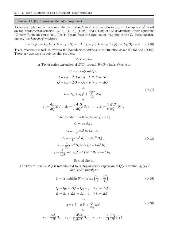
x = x{q(L = L 0 , B), p(L = L 0 , B)} = rB , y = y{q(L = L 0 , B), p(L = L 0 , B)} = 0 . (D.46)
There remains the task to express the boundary conditions in the function space (D.15) and (D.16).
There are two ways in solving this problem.
First choice.
A Taylor series expansion of B(Q) around B 0 (Q 0 ) leads directly to
B = arcsin(tanh Q) ,
B = B 0 + ∆B = B 0 + b ∀ b := ∆B ,
Q = Q 0 + ∆Q = Q 0 + q ∀ q := ∆Q
⇒
b = d 1 q + d 2 q
2 +
N →∞
r=3
d r q
r
∀
d 1 =
dB
dQ
(Q 0 ) , d 2 =
1
2!
d
2 B
dQ 2 (Q 0 ) , · · · , d r =
1
r!
d
r B
dQ r (Q 0 ) .
(D.47)
The standard coefficients are given by
d 1 = cos B 0 ,
d 2 = −
1
2
cos
2 B 0 tan B 0 ,
d 3 = −
1
6
cos
3 B 0 [1 − tan
2 B 0 ] ,
d 4 =
1
24
cos
4 B 0 tan B 0 [5 − tan
2 B 0 ] ,
d 5 =
1
120
cos
5 B 0 [5 − 18 tan
2 B 0 + tan
4 B 0 ] .
(D.48)
Second choice.
The first or remove step is materialized by a Taylor series expansion of Q(B) around Q 0 (B 0 )
and leads directly to
Q = artanh(sin B) = ln tan
π
4
+
B
2
,
(D.49)
Q = Q 0 + ∆Q = Q 0 + q ∀ q := ∆Q ,
B = B 0 + ∆B = B 0 + b ∀ b := ∆B
⇒
q = c 1 b + c 2 b
2 +
∞
r=3
c r b
r
∀
c 1 =
dQ
dB
(B 0 ) , c 2 =
1
2!
d
2 Q
dB 2 (B 0 ) , · · · , c r =
1
r!
d
r Q
dB r (B 0 ) .
(D.50)
Example D.1 (S
2
r , transverse Mercator projection).
As an example, let us construct the transverse Mercator projection locally for the sphere S
2
r based
on the fundamental solution (D.15), (D.16), (D.28), and (D.29) of the d’Alembert–Euler equations
(Cauchy–Riemann equations). Let us depart from the equidistant mapping of the L 0 meta-equator,
namely the boundary condition
x = x{q(L = L 0 , B), p(L = L 0 , B)} = rB , y = y{q(L = L 0 , B), p(L = L 0 , B)} = 0 . (D.46)
There remains the task to express the boundary conditions in the function space (D.15) and (D.16).
There are two ways in solving this problem.
First choice.
A Taylor series expansion of B(Q) around B 0 (Q 0 ) leads directly to
B = arcsin(tanh Q) ,
B = B 0 + ∆B = B 0 + b ∀ b := ∆B ,
Q = Q 0 + ∆Q = Q 0 + q ∀ q := ∆Q
⇒
b = d 1 q + d 2 q
2 +
N →∞
r=3
d r q
r
∀
d 1 =
dB
dQ
(Q 0 ) , d 2 =
1
2!
d
2 B
dQ 2 (Q 0 ) , · · · , d r =
1
r!
d
r B
dQ r (Q 0 ) .
(D.47)
The standard coefficients are given by
d 1 = cos B 0 ,
d 2 = −
1
2
cos
2 B 0 tan B 0 ,
d 3 = −
1
6
cos
3 B 0 [1 − tan
2 B 0 ] ,
d 4 =
1
24
cos
4 B 0 tan B 0 [5 − tan
2 B 0 ] ,
d 5 =
1
120
cos
5 B 0 [5 − 18 tan
2 B 0 + tan
4 B 0 ] .
(D.48)
Second choice.
The first or remove step is materialized by a Taylor series expansion of Q(B) around Q 0 (B 0 )
and leads directly to
Q = artanh(sin B) = ln tan
π
4
+
B
2
,
(D.49)
Q = Q 0 + ∆Q = Q 0 + q ∀ q := ∆Q ,
B = B 0 + ∆B = B 0 + b ∀ b := ∆B
⇒
q = c 1 b + c 2 b
2 +
∞
r=3
c r b
r
∀
c 1 =
dQ
dB
(B 0 ) , c 2 =
1
2!
d
2 Q
dB 2 (B 0 ) , · · · , c r =
1
r!
d
r Q
dB r (B 0 ) .
(D.50)