

D-2 D’Alembert–Euler (Cauchy–Riemann) equations 529
D-2 D’Alembert–Euler (Cauchy–Riemann) equations
Once an isometric coordinate system of a two-dimensional Riemann manifold {M
2 , λ
−2 δ µν } (“surface”)
has been established, an alternative isometric coordinate system can be constructed by solving a
boundary value problem of the d’Alembert–Euler equations (Cauchy–Riemann equations) subject to
the integrability conditions of harmonicity type. Here, we are going to construct fundamental solutions
of these basic equations governing conformal mapping.
Lemma D.2 (Fundamental solution of the d’Alembert–Euler equations subject to integrability conditions
of harmonicity, polynomial representation).
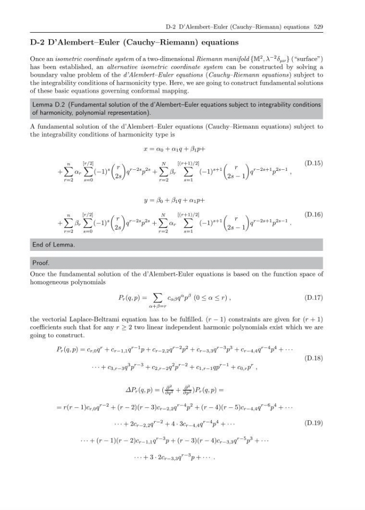
A fundamental solution of the d’Alembert–Euler equations (Cauchy–Riemann equations) subject to
the integrability conditions of harmonicity type is
x = α 0 + α 1 q + β 1 p+
+
n
r=2
α r
[r/2]
s=0
(−1)
s
r
2s
q
r−2s p
2s +
N
r=2
β r
[(r+1)/2]
s=1
(−1)
s+1
r
2s − 1
q
r−2s+1 p
2s−1 ,
(D.15)
y = β 0 + β 1 q + α 1 p+
+
n
r=2
β r
[r/2]
s=0
(−1)
s
r
2s
q
r−2s p
2s +
N
r=2
α r
[(r+1)/2]
s=1
(−1)
s+1
r
2s − 1
q
r−2s+1 p
2s−1 .
(D.16)
End of Lemma.
Proof.
Once the fundamental solution of the d’Alembert-Euler equations is based on the function space of
homogeneous polynomials
P r (q, p) =
α+β=r
c αβ q
α p
β (0 ≤ α ≤ r) ,
(D.17)
the vectorial Laplace-Beltrami equation has to be fulfilled. (r − 1) constraints are given for (r + 1)
coefficients such that for any r ≥ 2 two linear independent harmonic polynomials exist which we are
going to construct.
P r (q, p) = c r,0 q
r + c r−1,1 q
r−1 p + c r−2,2 q
r−2 p
2 + c r−3,3 q
r−3 p
3 + c r−4,4 q
r−4 p
4 + · · ·
· · · + c 3,r−3 q
3 p
r−3 + c 2,r−2 q
2 p
r−2 + c 1,r−1 qp
r−1 + c 0,r p
r ,
(D.18)
∆P r (q, p) = (
∂
2
∂q 2 +
∂
2
∂p 2 )P r (q, p) =
= r(r − 1)c r,0 q
r−2 + (r − 2)(r − 3)c r−2,2 q
r−4 p
2 + (r − 4)(r − 5)c r−4,4 q
r−6 p
4 + · · ·
· · · + 2c r−2,2 q
r−2 + 4 · 3c r−4,4 q
r−4 p
4 + · · ·
· · · + (r − 1)(r − 2)c r−1,1 q
r−3 p + (r − 3)(r − 4)c r−3,3 q
r−5 p
3 + · · ·
· · · + 3 · 2c r−3,3 q
r−3 p + · · · .
(D.19)
D-2 D’Alembert–Euler (Cauchy–Riemann) equations
Once an isometric coordinate system of a two-dimensional Riemann manifold {M
2 , λ
−2 δ µν } (“surface”)
has been established, an alternative isometric coordinate system can be constructed by solving a
boundary value problem of the d’Alembert–Euler equations (Cauchy–Riemann equations) subject to
the integrability conditions of harmonicity type. Here, we are going to construct fundamental solutions
of these basic equations governing conformal mapping.
Lemma D.2 (Fundamental solution of the d’Alembert–Euler equations subject to integrability conditions
of harmonicity, polynomial representation).
A fundamental solution of the d’Alembert–Euler equations (Cauchy–Riemann equations) subject to
the integrability conditions of harmonicity type is
x = α 0 + α 1 q + β 1 p+
+
n
r=2
α r
[r/2]
s=0
(−1)
s
r
2s
q
r−2s p
2s +
N
r=2
β r
[(r+1)/2]
s=1
(−1)
s+1
r
2s − 1
q
r−2s+1 p
2s−1 ,
(D.15)
y = β 0 + β 1 q + α 1 p+
+
n
r=2
β r
[r/2]
s=0
(−1)
s
r
2s
q
r−2s p
2s +
N
r=2
α r
[(r+1)/2]
s=1
(−1)
s+1
r
2s − 1
q
r−2s+1 p
2s−1 .
(D.16)
End of Lemma.
Proof.
Once the fundamental solution of the d’Alembert-Euler equations is based on the function space of
homogeneous polynomials
P r (q, p) =
α+β=r
c αβ q
α p
β (0 ≤ α ≤ r) ,
(D.17)
the vectorial Laplace-Beltrami equation has to be fulfilled. (r − 1) constraints are given for (r + 1)
coefficients such that for any r ≥ 2 two linear independent harmonic polynomials exist which we are
going to construct.
P r (q, p) = c r,0 q
r + c r−1,1 q
r−1 p + c r−2,2 q
r−2 p
2 + c r−3,3 q
r−3 p
3 + c r−4,4 q
r−4 p
4 + · · ·
· · · + c 3,r−3 q
3 p
r−3 + c 2,r−2 q
2 p
r−2 + c 1,r−1 qp
r−1 + c 0,r p
r ,
(D.18)
∆P r (q, p) = (
∂
2
∂q 2 +
∂
2
∂p 2 )P r (q, p) =
= r(r − 1)c r,0 q
r−2 + (r − 2)(r − 3)c r−2,2 q
r−4 p
2 + (r − 4)(r − 5)c r−4,4 q
r−6 p
4 + · · ·
· · · + 2c r−2,2 q
r−2 + 4 · 3c r−4,4 q
r−4 p
4 + · · ·
· · · + (r − 1)(r − 2)c r−1,1 q
r−3 p + (r − 3)(r − 4)c r−3,3 q
r−5 p
3 + · · ·
· · · + 3 · 2c r−3,3 q
r−3 p + · · · .
(D.19)