

32
1 From Riemann manifolds to Riemann manifolds
∂/∂U
∂/∂V
√ κ 1
√ κ 2
∂/∂u
1
∂/∂v
1
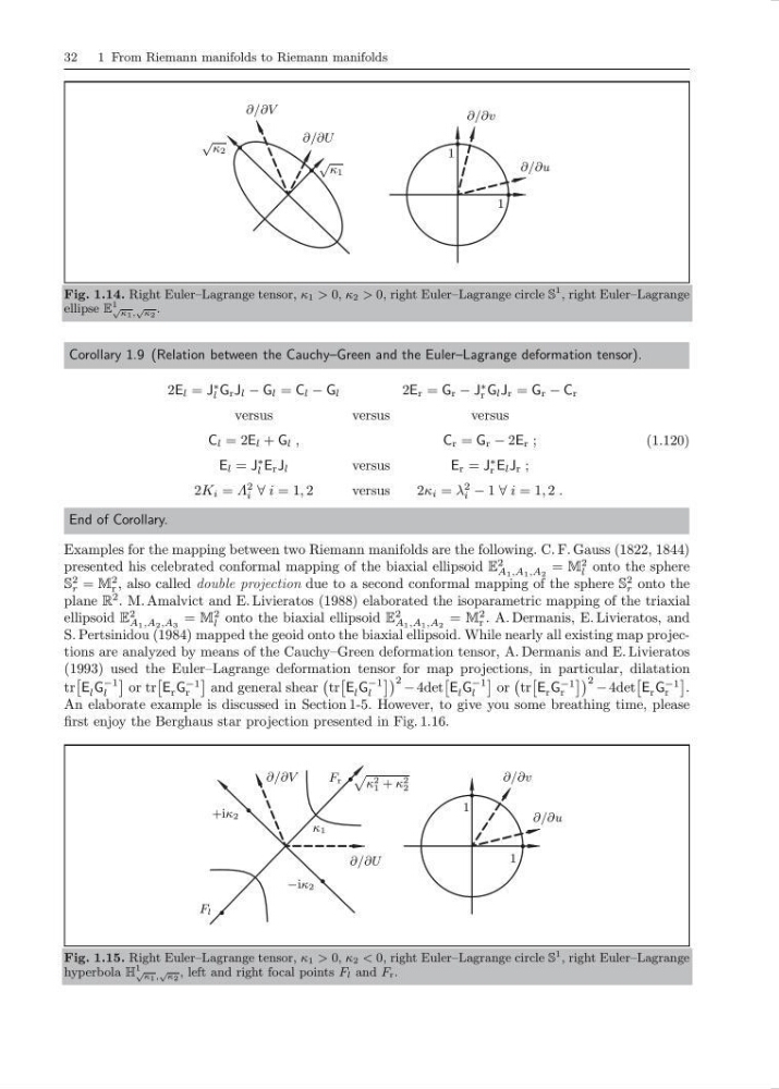
Fig. 1.14. Right Euler–Lagrange tensor, κ 1 > 0, κ 2 > 0, right Euler–Lagrange circle S
1 , right Euler–Lagrange
ellipse E
1 √ κ 1 ,
√
κ 2
.
Corollary 1.9 (Relation between the Cauchy–Green and the Euler–Lagrange deformation tensor).
2E l = J
∗
l G r J l − G l = C l − G l
2E r = G r − J
∗
r G l J r = G r − C r
versus
versus
versus
C l = 2E l + G l ,
C r = G r − 2E r ;
E l = J
∗
l E r J l
versus
E r = J
∗
r E l J r ;
2K i = Λ
2
i ∀ i = 1, 2
v ersus
2κ i = λ
2
i − 1 ∀ i = 1, 2 .
(1.120)
End of Corollary.
Examples for the mapping between two Riemann manifolds are the following. C. F. Gauss (1822, 1844)
presented his celebrated conformal mapping of the biaxial ellipsoid E
2
A 1 ,A 1 ,A 2
= M
2
l onto the sphere
S
2
r = M
2
r , also called double projection due to a second conformal mapping of the sphere S
2
r onto the
plane R
2 . M. Amalvict and E. Livieratos (1988) elaborated the isoparametric mapping of the triaxial
ellipsoid E
2
A 1 ,A 2 ,A 3
= M
2
l onto the biaxial ellipsoid E
2
A 1 ,A 1 ,A 2
= M
2
r . A. Dermanis, E. Livieratos, and
S. Pertsinidou (1984) mapped the geoid onto the biaxial ellipsoid. While nearly all existing map projections are analyzed by means of the Cauchy–Green deformation tensor, A. Dermanis and E. Livieratos
(1993) used the Euler–Lagrange deformation tensor for map projections, in particular, dilatation
tr
E l G
−1
l
or tr
E r G
−1
r
and general shear
tr
E l G
−1
l
2 − 4det
E l G
−1
l
or
tr
E r G
−1
r
2 − 4det
E r G
−1
r
.
An elaborate example is discussed in Section 1-5. However, to give you some breathing time, please
first enjoy the Berghaus star projection presented in Fig. 1.16.
∂/∂U
∂/∂V
p
κ
2
1 + κ
2
2
+iκ 2
−iκ 2
F r
F l
κ 1
∂/∂u
1
∂/∂v
1
Fig. 1.15. Right Euler–Lagrange tensor, κ 1 > 0, κ 2 < 0, right Euler–Lagrange circle S
1 , right Euler–Lagrange
hyperbola H
1 √
κ 1 ,
√
κ 2
, left and right focal points F l and F r .
1 From Riemann manifolds to Riemann manifolds
∂/∂U
∂/∂V
√ κ 1
√ κ 2
∂/∂u
1
∂/∂v
1
Fig. 1.14. Right Euler–Lagrange tensor, κ 1 > 0, κ 2 > 0, right Euler–Lagrange circle S
1 , right Euler–Lagrange
ellipse E
1 √ κ 1 ,
√
κ 2
.
Corollary 1.9 (Relation between the Cauchy–Green and the Euler–Lagrange deformation tensor).
2E l = J
∗
l G r J l − G l = C l − G l
2E r = G r − J
∗
r G l J r = G r − C r
versus
versus
versus
C l = 2E l + G l ,
C r = G r − 2E r ;
E l = J
∗
l E r J l
versus
E r = J
∗
r E l J r ;
2K i = Λ
2
i ∀ i = 1, 2
v ersus
2κ i = λ
2
i − 1 ∀ i = 1, 2 .
(1.120)
End of Corollary.
Examples for the mapping between two Riemann manifolds are the following. C. F. Gauss (1822, 1844)
presented his celebrated conformal mapping of the biaxial ellipsoid E
2
A 1 ,A 1 ,A 2
= M
2
l onto the sphere
S
2
r = M
2
r , also called double projection due to a second conformal mapping of the sphere S
2
r onto the
plane R
2 . M. Amalvict and E. Livieratos (1988) elaborated the isoparametric mapping of the triaxial
ellipsoid E
2
A 1 ,A 2 ,A 3
= M
2
l onto the biaxial ellipsoid E
2
A 1 ,A 1 ,A 2
= M
2
r . A. Dermanis, E. Livieratos, and
S. Pertsinidou (1984) mapped the geoid onto the biaxial ellipsoid. While nearly all existing map projections are analyzed by means of the Cauchy–Green deformation tensor, A. Dermanis and E. Livieratos
(1993) used the Euler–Lagrange deformation tensor for map projections, in particular, dilatation
tr
E l G
−1
l
or tr
E r G
−1
r
and general shear
tr
E l G
−1
l
2 − 4det
E l G
−1
l
or
tr
E r G
−1
r
2 − 4det
E r G
−1
r
.
An elaborate example is discussed in Section 1-5. However, to give you some breathing time, please
first enjoy the Berghaus star projection presented in Fig. 1.16.
∂/∂U
∂/∂V
p
κ
2
1 + κ
2
2
+iκ 2
−iκ 2
F r
F l
κ 1
∂/∂u
1
∂/∂v
1
Fig. 1.15. Right Euler–Lagrange tensor, κ 1 > 0, κ 2 < 0, right Euler–Lagrange circle S
1 , right Euler–Lagrange
hyperbola H
1 √
κ 1 ,
√
κ 2
, left and right focal points F l and F r .