440 20 Geodetic mapping
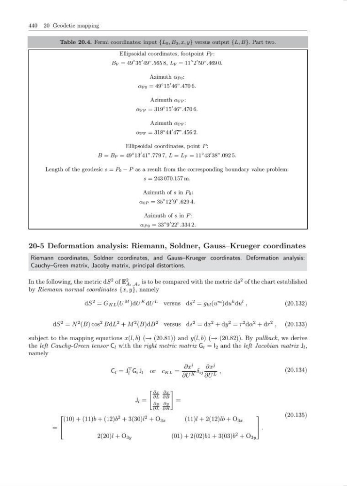
Table 20.4. Fermi coordinates: input {L 0 , B 0 , x, y} versus output {L, B}. Part two.
Ellipsoidal coordinates, footpoint P F :
B F = 49
◦ 36
49”.565 8, L F = 11
◦ 2
50”.469 0.
Azimuth α F0 :
α F0 = 49
◦ 15
46”.470 6.
Azimuth α FP :
α FP = 319
◦ 15
46”.470 6.
Azimuth α PF :
α PF = 318
◦ 44
47”.456 2.
Ellipsoidal coordinates, point P :
B = B P = 49
◦ 13
41”.779 7, L = L P = 11
◦ 43
38”.092 5.
Length of the geodesic s = P 0 − P as a result from the corresponding boundary value problem:
s = 243 070.157 m.
Azimuth of s in P 0 :
α 0P = 35
◦ 12
9”.629 4.
Azimuth of s in P :
α P 0 = 33
◦ 9
22”.334 2.
20-5 Deformation analysis: Riemann, Soldner, Gauss–Krueger coordinates
Riemann coordinates, Soldner coordinates, and Gauss–Krueger coordinates. Deformation analysis:
Cauchy–Green matrix, Jacoby matrix, principal distortions.
In the following, the metric dS
2 of E
2
A 1 ,A 2
is to be compared with the metric ds
2 of the chart established
by Riemann normal coordinates {x, y}, namely
dS
2 = G KL (U
M )dU
K dU
L versus ds
2 = g kl (u
m )du
k du
l ,
(20.132)
dS
2 = N
2 (B) cos
2 BdL
2 + M
2 (B)dB
2 versus ds
2 = dx
2 + dy
2 = r
2 dα
2 + dr
2 , (20.133)
subject to the mapping equations x(l, b) (→ (20.81)) and y(l, b) (→ (20.82)). By pullback, we derive
the left Cauchy-Green tensor C l with the right metric matrix G r = I 2 and the left Jacobian matrix J l ,
namely
C l = J
T
l G r J l or c KL =
∂x
i
∂U K δ ij
∂x
j
∂U L ,
(20.134)
J l =
∂x
∂L
∂x
∂B
∂y
∂L
∂y
∂B
=
=
⎡
⎣
(10) + (11)b + (12)b
2 + 3(30)l
2 + O 3x
(11)l + 2(12)lb + O 3x
2(20)l + O 3y
(01) + 2(02)b1 + 3(03)b
2 + O 3y
⎤
⎦ .
(20.135)