

20-4 Fermi coordinates: oblique geodetic parallel coordinates 439
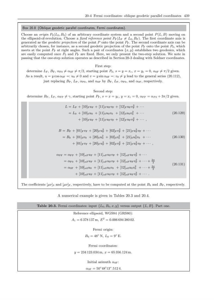
Box 20.8 (Oblique geodetic parallel coordinates, Fermi coordinates).
Choose an origin P 0 (L 0 , B 0 ) of an arbitrary coordinate system and a second point P (L, B) moving on
the ellipsoid-of-revolution. Choose a fixed reference point P F (L F = L 0 , B F ). The first coordinate axis is
generated as the geodetic projection of the point P onto the point P F . The second coordinate axis can be
arbitrarily chosen, for instance, as a second geodetic projection of the point P F onto the point P 0 , which
meets at the point P F at right angles. Such a pair of coordinates {x, y} establishes two geodesics, which
are easily computed once P 0 and P F are fixed. Here, we only present the two-step solution. We note in
passing that the one-step solution operates as described in Section 20-3 dealing with Soldner coordinates.
First step:
determine L F , B F , α F0 = α 0F = π/2, starting point P 0 , s = y = x c , x = y c = 0, α 0F = π/2 given.
As a result, u = y cos α 0F =: u 0 = 0 and v = y sin α 0F =: v 0 = y lead to the general series (20.112),
just replacing B P , L P , α P0 , and α 0P by B F , L F , α F0 , and α 0F , respectively.
Second step:
determine B F , L F , α FP = γ, starting point P F , s = x = y c , y = x c = 0, α FP = α F 0 + 3π/2 given.
L = L F + [10] F u F + [11] F u F v F + [12] F u F v
2
F + · · ·
= L 0 + [10] 0 u 0 + [11] 0 u 0 v 0 + [12] 0 u 0 v
2
0 + · · ·
+ [10] F u F + [11] F u F v F + [12] F u F v
2
F + · · · ,
(20.129)
B = B F + [01] F v F + [20] F u
2
F + [02] F v
2
F + [21] F u
2
F v F + · · ·
= B 0 + [01] 0 v 0 + [20] 0 u
2
0 + [02] 0 v
2
0 + [21] 0 u
2
0 v 0 + · · ·
+ [01] F v F + [20] F u
2
F + [02] F v
2
F + [21] F u
2
F v F + · · · ,
(20.130)
α PF = α FP + [10] αF u F + [11] αF u F v F + [12] αF u F v
2
F + · · ·
= α F0 + [10] αF u F + [11] αF u F v F + [12] αF u F v
2
F + · · · +
3π
2
= α 0F + [10] α0 u 0 + [11] α0 u 0 v 0 + [12] α0 u 0 v
2
0 + · · · +
3π
2
+ [10] αF u F + [11] αF u F v F + [12] αF u F v
2
F + · · · .
(20.131)
The coefficients [µν] 0 and [µν] F , respectively, have to be computed at the point B 0 and B F , respectively.
A numerical example is given in Tables 20.3 and 20.4.
Table 20.3. Fermi coordinates: input {L 0 , B 0 , x, y} versus output {L, B}. Part one.
Reference ellipsoid, WGS84 (GRS80):
A 1 = 6 378 137 m, E
2 = 0.006 694 380 02.
Fermi origin:
B 0 = 48
◦ N, L 0 = 9
◦ E.
Fermi coordinates:
y = 234 123.034 m, x = 65 356.124 m.
Initial azimuth α 0F :
α 0F = 50
◦ 48
13”.512 4.
Box 20.8 (Oblique geodetic parallel coordinates, Fermi coordinates).
Choose an origin P 0 (L 0 , B 0 ) of an arbitrary coordinate system and a second point P (L, B) moving on
the ellipsoid-of-revolution. Choose a fixed reference point P F (L F = L 0 , B F ). The first coordinate axis is
generated as the geodetic projection of the point P onto the point P F . The second coordinate axis can be
arbitrarily chosen, for instance, as a second geodetic projection of the point P F onto the point P 0 , which
meets at the point P F at right angles. Such a pair of coordinates {x, y} establishes two geodesics, which
are easily computed once P 0 and P F are fixed. Here, we only present the two-step solution. We note in
passing that the one-step solution operates as described in Section 20-3 dealing with Soldner coordinates.
First step:
determine L F , B F , α F0 = α 0F = π/2, starting point P 0 , s = y = x c , x = y c = 0, α 0F = π/2 given.
As a result, u = y cos α 0F =: u 0 = 0 and v = y sin α 0F =: v 0 = y lead to the general series (20.112),
just replacing B P , L P , α P0 , and α 0P by B F , L F , α F0 , and α 0F , respectively.
Second step:
determine B F , L F , α FP = γ, starting point P F , s = x = y c , y = x c = 0, α FP = α F 0 + 3π/2 given.
L = L F + [10] F u F + [11] F u F v F + [12] F u F v
2
F + · · ·
= L 0 + [10] 0 u 0 + [11] 0 u 0 v 0 + [12] 0 u 0 v
2
0 + · · ·
+ [10] F u F + [11] F u F v F + [12] F u F v
2
F + · · · ,
(20.129)
B = B F + [01] F v F + [20] F u
2
F + [02] F v
2
F + [21] F u
2
F v F + · · ·
= B 0 + [01] 0 v 0 + [20] 0 u
2
0 + [02] 0 v
2
0 + [21] 0 u
2
0 v 0 + · · ·
+ [01] F v F + [20] F u
2
F + [02] F v
2
F + [21] F u
2
F v F + · · · ,
(20.130)
α PF = α FP + [10] αF u F + [11] αF u F v F + [12] αF u F v
2
F + · · ·
= α F0 + [10] αF u F + [11] αF u F v F + [12] αF u F v
2
F + · · · +
3π
2
= α 0F + [10] α0 u 0 + [11] α0 u 0 v 0 + [12] α0 u 0 v
2
0 + · · · +
3π
2
+ [10] αF u F + [11] αF u F v F + [12] αF u F v
2
F + · · · .
(20.131)
The coefficients [µν] 0 and [µν] F , respectively, have to be computed at the point B 0 and B F , respectively.
A numerical example is given in Tables 20.3 and 20.4.
Table 20.3. Fermi coordinates: input {L 0 , B 0 , x, y} versus output {L, B}. Part one.
Reference ellipsoid, WGS84 (GRS80):
A 1 = 6 378 137 m, E
2 = 0.006 694 380 02.
Fermi origin:
B 0 = 48
◦ N, L 0 = 9
◦ E.
Fermi coordinates:
y = 234 123.034 m, x = 65 356.124 m.
Initial azimuth α 0F :
α 0F = 50
◦ 48
13”.512 4.