

438 20 Geodetic mapping
20-32 Second problem of Soldner coordinates: geodetic parallel coordinates, input
{L, B, L 0 , B 0 } versus output {x = y c , y = x c }
The inverse problem to derive the Soldner coordinates {x = y c , y = x c } from the given values of
{L, B, L 0 , B 0 } is again solved by series inversion, the result of which is provided by (20.127) and
(20.128), with (µν)
S
x and (µν)
S
y as Soldner inverse series coefficients.
x =
∞
µ=0
∞
ν=0
(µν)
S
x (B − B 0 )
µ (L − L 0 )
ν ,
(20.127)
y =
∞
µ=0
∞
ν=0
(µν)
S
y (B − B 0 )
µ (L − L 0 )
ν .
(20.128)
20-4 Fermi coordinates: oblique geodetic parallel coordinates
Fermi coordinates: oblique geodetic parallel coordinates. Geodetic projection. The two-step solution and
the two-step solution equations.
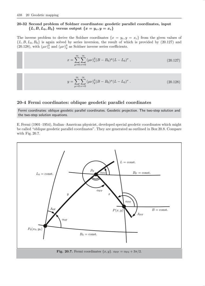
E. Fermi (1901–1954), Italian–American physicist, developed special geodetic coordinates which might
be called “oblique geodetic parallel coordinates”. They are generated as outlined in Box 20.8. Compare
with Fig. 20.7.
P F
α F0
α FP
x
y
L 0 = const.
B F = const.
A 0F
B 0 = const.
α 0F
L = const.
A PF
α PF
P (x, y)
B = const.
P 0 (x 0 , y 0 )
Fig. 20.7. Fermi coordinates {x, y}. α FP = α F0 + 3π/2.
20-32 Second problem of Soldner coordinates: geodetic parallel coordinates, input
{L, B, L 0 , B 0 } versus output {x = y c , y = x c }
The inverse problem to derive the Soldner coordinates {x = y c , y = x c } from the given values of
{L, B, L 0 , B 0 } is again solved by series inversion, the result of which is provided by (20.127) and
(20.128), with (µν)
S
x and (µν)
S
y as Soldner inverse series coefficients.
x =
∞
µ=0
∞
ν=0
(µν)
S
x (B − B 0 )
µ (L − L 0 )
ν ,
(20.127)
y =
∞
µ=0
∞
ν=0
(µν)
S
y (B − B 0 )
µ (L − L 0 )
ν .
(20.128)
20-4 Fermi coordinates: oblique geodetic parallel coordinates
Fermi coordinates: oblique geodetic parallel coordinates. Geodetic projection. The two-step solution and
the two-step solution equations.
E. Fermi (1901–1954), Italian–American physicist, developed special geodetic coordinates which might
be called “oblique geodetic parallel coordinates”. They are generated as outlined in Box 20.8. Compare
with Fig. 20.7.
P F
α F0
α FP
x
y
L 0 = const.
B F = const.
A 0F
B 0 = const.
α 0F
L = const.
A PF
α PF
P (x, y)
B = const.
P 0 (x 0 , y 0 )
Fig. 20.7. Fermi coordinates {x, y}. α FP = α F0 + 3π/2.