20-5 Deformation analysis: Riemann, Soldner, Gauss–Krueger coordinates 441
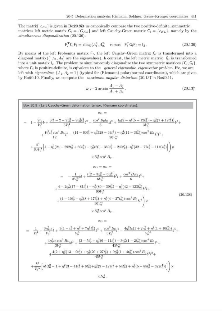
The matrix[ c KL ] is given in Box 20.9 . L et us canonically compare the two positive-definite, symmetric
matrices left metric matrix G l = {G KL } and left Cauchy-Green matrix C l = {c KL }, namely by the
simultaneous diagonalization (20.136).
F
T
l C l F l = diag (Λ
2
1 , Λ
2
2 ) versus F
T
l G l F l = I 2 .
(20.136)
By means of the left Frobenius matrix F l , the left Cauchy–Green matrix C l is transformed into a
diagonal matrix , (( Λ 1 , Λ 2 ) are the eigenvalues). I
n contrast, the left metric matrix G l is transformed
into a unit matrix I 2 . The problem to simultaneously diagonalize the two symmetric matrices {C l , G l },
where G l is positive-definite, is eq uivalent to the general eigenvalue–eigenvector problem. H ere, we are
left with eigenvalues {Λ 1 , Λ 2 = 1} (typical for (Riemann) polar/normal coordinates), which are given
by Box 20.10. Finally, we compute the maximum angular distortion (20.137 ) in Box 20.11.
ω := 2 arcsin
Λ 1 − Λ 2
Λ 1 + Λ 2
.
(20.137 )
Box 20.9 (Left Cauchy–Green deformation tensor, Riemann coordinates).
c 11 =
= 1 −
2t 0
V
2
0
b +
3t
2
0 − 2 − 2η
2
0 − 9η
2
0 t
2
0
3V
4
0
b
2 −
cos
2 B 0 t 0
3
bl
2 +
t 0 (2 − η
2
0 (5 + 12t
2
0 ) − η
4
0 (7 + 12t
2
0 ))
3V
6
0
b
3 +
+
V
2
0 t
2
0 cos
4 B 0
12
l
4 −
(14 − 60t
2
0 + η
2
0 (28 − 63t
2
0 ) + η
4
0 (14 − 3t
2
0 )) cos
2 B 0
90V
4
0
b
2 l
2 +
+
b
4
60V
8
0
h
4 − η
2
0 (24 − 292t
2
0 + 60t
4
0 ) − η
4
0 (60 − 369t
2
0 − 240t
4
0 )−η
6
0 (32 − 77t
2
0 − 1140t
4
0 )
i
!
×
×N
2
0 cos
2 B 0 ,
c 12 = c 21 =
= −
1
3V
2
0
bl +
t(2 − 3η
2
0 − 5η
4
0 )
6V
6
0
b
2 l +
cos
2 B 0 t 0
6
l
3 +
+
4 − 2η
2
0 (17 − 81t
2
0 ) − η
4
0 (80 − 39t
2
0 ) − η
6
0 (42 + 123t
2
0 )
90V
8
0
b
3 l+
+
(4 − 10t
2
0 + η
2
0 (8 + 17t
2
0 ) + η
4
0 (4 + 27t
2
0 )) cos
2 B 0
90V
4
0
bl
3
!
×
×N
2
0 cos
2 B 0 ,
c 22 =
=
1
V
4
0
+
6η
2
0 t 0
V
6
0
b +
3(1 − t
2
0 + η
2
0 + 7η
2
0 t
2
0 )
V
8
0
b
2 +
cos
2 B 0
3V
2
0
l
2 −
4η
2
0 t 0 (1 + 2η
2
0 + η
4
0 (1 + 10t
2
0 ))
V
10
0
b
3 +
+
4η
2
0 t 0 cos
2 B 0
3V
4
0
bl
2 +
(3 − 5t
2
0 + η
2
0 (6 − 11t
2
0 ) + 3η
4
0 (1 − 2t
2
0 )) cos
4 B 0
45V
4
0
l
4 +
+
4(2 + η
2
0 (13 − 9t
2
0 ) + η
4
0 (20 + 27t
2
0 ) + 9η
6
0 (1 + 4t
2
0 )) cos
2 B 0
45V
8
0
b
2 l
2 +
+
b
4
V
12
0
h
η
2
0 (t
2
0 − 1 + η
2
0 (3 − 41t
2
0 + 6t
4
0 )+η
4
0 (9 − 127t
2
0 + 54t
4
0 ) + η
6
0 (5 − 85t
2
0 − 522t
4
0 ))
i
!
×
×N
2
0 .
(20.138)