

20-1 Geodesic, geodesic circle, Darboux frame, Riemann coordinates 425
S
N
C 2 (N or th )
C 1 (E as t)
P 0
y
x
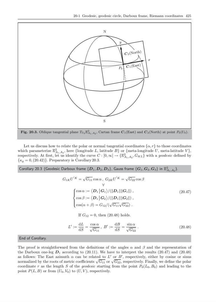
Fig. 20.3. Oblique tangential plane T U 0 E
2
A 1 ,A 2 , Cartan frame C 1 (East) and C 2 (North) at point P 0 (U 0 ).
Let us discuss how to relate the polar or normal tangential coordinates {α, r} to those coordinates
which parameterize E
2
A 1 ,A 2
, here {longitude L, latitude B} or {meta-longitude U , meta-latitude V },
respectively. At first, let us identify the curve C : [0, ∞] → {E
2
A 1 ,A 2
, G KL } with a geodesic defined by
{κ g = 0, (20.42)}. Preparatory is Corollary 20.3.
Corollary 20.3 (Geodesic Darboux frame {D 1 , D 2 , D 3 }, Gauss frame {G 1 , G 2 , G 3 } in E
2
A 1 ,A 2
).
G 1K U
K =
√
G 11 cos α , G 2K U
K =
√
G 22 cos β
∀
⎧
⎪ ⎪ ⎨
⎪ ⎪ ⎩
cos α :=
D 1 G 1
/(D 1 1 ) ,
cos β :=
D 1 G 2
/(D 1 2 ) ,
cos(α + β) = G 12 /(
√
G 11
√
G 22 ) .
(20.47)
If G 12 = 0, then (20.48) holds.
L
:=
dL
dS
=
cos α
√
G 11
, B
:=
dB
dS
=
sin α
√
G 22
.
(20.48)
End of Corollary.
The proof is straightforward from the definitions of the angles α and β and the representation of
the Darboux one-leg D 1 according to (20.11). We have to interpret the results (20.47) and (20.48)
as follows: The East azimuth α can be related to L
or B
, respectively, either by cosine or sinus
normalized by the roots of metric coefficients
√
G 11 or
√
G 22 , respectively. Finally, we define the polar
coordinate r as the length S of the geodesic starting from the point P 0 (L 0 , B 0 ) and leading to the
point P (L, B) or from (U 0 , V 0 ) to (U, V ), respectively.
S
N
C 2 (N or th )
C 1 (E as t)
P 0
y
x
Fig. 20.3. Oblique tangential plane T U 0 E
2
A 1 ,A 2 , Cartan frame C 1 (East) and C 2 (North) at point P 0 (U 0 ).
Let us discuss how to relate the polar or normal tangential coordinates {α, r} to those coordinates
which parameterize E
2
A 1 ,A 2
, here {longitude L, latitude B} or {meta-longitude U , meta-latitude V },
respectively. At first, let us identify the curve C : [0, ∞] → {E
2
A 1 ,A 2
, G KL } with a geodesic defined by
{κ g = 0, (20.42)}. Preparatory is Corollary 20.3.
Corollary 20.3 (Geodesic Darboux frame {D 1 , D 2 , D 3 }, Gauss frame {G 1 , G 2 , G 3 } in E
2
A 1 ,A 2
).
G 1K U
K =
√
G 11 cos α , G 2K U
K =
√
G 22 cos β
∀
⎧
⎪ ⎪ ⎨
⎪ ⎪ ⎩
cos α :=
D 1 G 1
/(D 1 1 ) ,
cos β :=
D 1 G 2
/(D 1 2 ) ,
cos(α + β) = G 12 /(
√
G 11
√
G 22 ) .
(20.47)
If G 12 = 0, then (20.48) holds.
L
:=
dL
dS
=
cos α
√
G 11
, B
:=
dB
dS
=
sin α
√
G 22
.
(20.48)
End of Corollary.
The proof is straightforward from the definitions of the angles α and β and the representation of
the Darboux one-leg D 1 according to (20.11). We have to interpret the results (20.47) and (20.48)
as follows: The East azimuth α can be related to L
or B
, respectively, either by cosine or sinus
normalized by the roots of metric coefficients
√
G 11 or
√
G 22 , respectively. Finally, we define the polar
coordinate r as the length S of the geodesic starting from the point P 0 (L 0 , B 0 ) and leading to the
point P (L, B) or from (U 0 , V 0 ) to (U, V ), respectively.