

426 20 Geodetic mapping
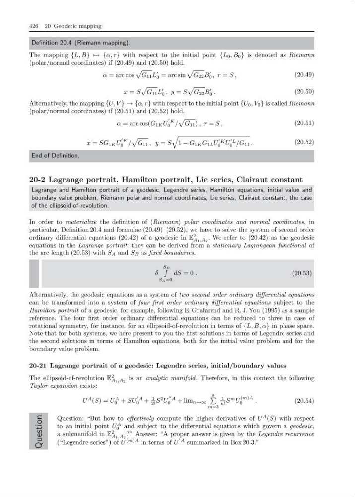
Definition 20.4 (Riemann mapping).
The mapping {L, B} → {α, r} with respect to the initial point {L 0 , B 0 } is denoted as Riemann
(polar/normal coordinates) if (20.49) and (20.50) hold.
α = arc cos
G 11 L
0 = arc sin
G 22 B
0 , r = S ,
(20.49)
x = S
G 11 L
0 , y = S
G 22 B
0 .
(20.50)
Alternatively, the mapping {U, V } → {α, r} with respect to the initial point {U 0 , V 0 } is called Riemann
(polar/normal coordinates) if (20.51) and (20.52) hold.
α = arc cos(G 1K U
K
0 /
G 11 ) , r = S ,
(20.51)
x = SG 1K U
K
0 /
G 11 , y = S
1 − G 1K G 1L U
K
0 U
L
0 /G 11 .
(20.52)
End of Definition.
20-2 Lagrange portrait, Hamilton portrait, Lie series, Clairaut constant
Lagrange and Hamilton portrait of a geodesic, Legendre series, Hamilton equations, initial value and
boundary value problem, Riemann polar and normal coordinates, Lie series, Clairaut constant, the case
of the ellipsoid-of-revolution.
In order to materialize the definition of (Riemann) polar coordinates and normal coordinates, in
particular, Definition 20.4 and formulae (20.49)–(20.52), we have to solve the system of second order
ordinary differential equations (20.42) of a geodesic in E
2
A 1 ,A 2
. We refer to (20.42) as the geodesic
equations in the Lagrange portrait: they can be derived from a stationary Lagrangean functional of
the arc length (20.53) with S A and S B as fixed boundaries.
δ
S B
S A =0
dS = 0 .
(20.53)
Alternatively, the geodesic equations as a system of two second order ordinary differential equations
can be transformed into a system of four first order ordinary differential equations subject to the
Hamilton portrait of a geodesic, for example, following E. Grafarend and R. J. You (1995) as a sample
reference. The four first order ordinary differential equations can be reduced to three in case of
rotational symmetry, for instance, for an ellipsoid-of-revolution in terms of {L, B, α} in phase space.
Note that for both systems, we here present to you the first solutions in terms of Legendre series and
the second solutions in terms of Hamilton equations, both for the initial value problem and for the
boundary value problem.
20-21 Lagrange portrait of a geodesic: Legendre series, initial/boundary values
The ellipsoid-of-revolution E
2
A 1 ,A 2
is an analytic manifold . Therefore, in this context the following
Taylor expansion exists:
U
A (S) = U
A
0 + SU
A
0 +
1
2! S
2 U
A
0
+ lim n→∞
n
m=3
1
n! S
m U
(m)A
0
.
(20.54)
Question.
Question: “But how to effectively compute the higher derivatives of U
A (S) with respect
to an initial point U
A
0 and subject to the differential equations which govern a geodesic,
a submanifold in E
2
A 1 ,A 2
?” Answer: “A proper answer is given by the Legendre recurrence
(“Legendre series”) of U
(m)A in terms of U
A summarized in Box 20.3.”
Definition 20.4 (Riemann mapping).
The mapping {L, B} → {α, r} with respect to the initial point {L 0 , B 0 } is denoted as Riemann
(polar/normal coordinates) if (20.49) and (20.50) hold.
α = arc cos
G 11 L
0 = arc sin
G 22 B
0 , r = S ,
(20.49)
x = S
G 11 L
0 , y = S
G 22 B
0 .
(20.50)
Alternatively, the mapping {U, V } → {α, r} with respect to the initial point {U 0 , V 0 } is called Riemann
(polar/normal coordinates) if (20.51) and (20.52) hold.
α = arc cos(G 1K U
K
0 /
G 11 ) , r = S ,
(20.51)
x = SG 1K U
K
0 /
G 11 , y = S
1 − G 1K G 1L U
K
0 U
L
0 /G 11 .
(20.52)
End of Definition.
20-2 Lagrange portrait, Hamilton portrait, Lie series, Clairaut constant
Lagrange and Hamilton portrait of a geodesic, Legendre series, Hamilton equations, initial value and
boundary value problem, Riemann polar and normal coordinates, Lie series, Clairaut constant, the case
of the ellipsoid-of-revolution.
In order to materialize the definition of (Riemann) polar coordinates and normal coordinates, in
particular, Definition 20.4 and formulae (20.49)–(20.52), we have to solve the system of second order
ordinary differential equations (20.42) of a geodesic in E
2
A 1 ,A 2
. We refer to (20.42) as the geodesic
equations in the Lagrange portrait: they can be derived from a stationary Lagrangean functional of
the arc length (20.53) with S A and S B as fixed boundaries.
δ
S B
S A =0
dS = 0 .
(20.53)
Alternatively, the geodesic equations as a system of two second order ordinary differential equations
can be transformed into a system of four first order ordinary differential equations subject to the
Hamilton portrait of a geodesic, for example, following E. Grafarend and R. J. You (1995) as a sample
reference. The four first order ordinary differential equations can be reduced to three in case of
rotational symmetry, for instance, for an ellipsoid-of-revolution in terms of {L, B, α} in phase space.
Note that for both systems, we here present to you the first solutions in terms of Legendre series and
the second solutions in terms of Hamilton equations, both for the initial value problem and for the
boundary value problem.
20-21 Lagrange portrait of a geodesic: Legendre series, initial/boundary values
The ellipsoid-of-revolution E
2
A 1 ,A 2
is an analytic manifold . Therefore, in this context the following
Taylor expansion exists:
U
A (S) = U
A
0 + SU
A
0 +
1
2! S
2 U
A
0
+ lim n→∞
n
m=3
1
n! S
m U
(m)A
0
.
(20.54)
Question.
Question: “But how to effectively compute the higher derivatives of U
A (S) with respect
to an initial point U
A
0 and subject to the differential equations which govern a geodesic,
a submanifold in E
2
A 1 ,A 2
?” Answer: “A proper answer is given by the Legendre recurrence
(“Legendre series”) of U
(m)A in terms of U
A summarized in Box 20.3.”