

17-2 Special mapping equations 391
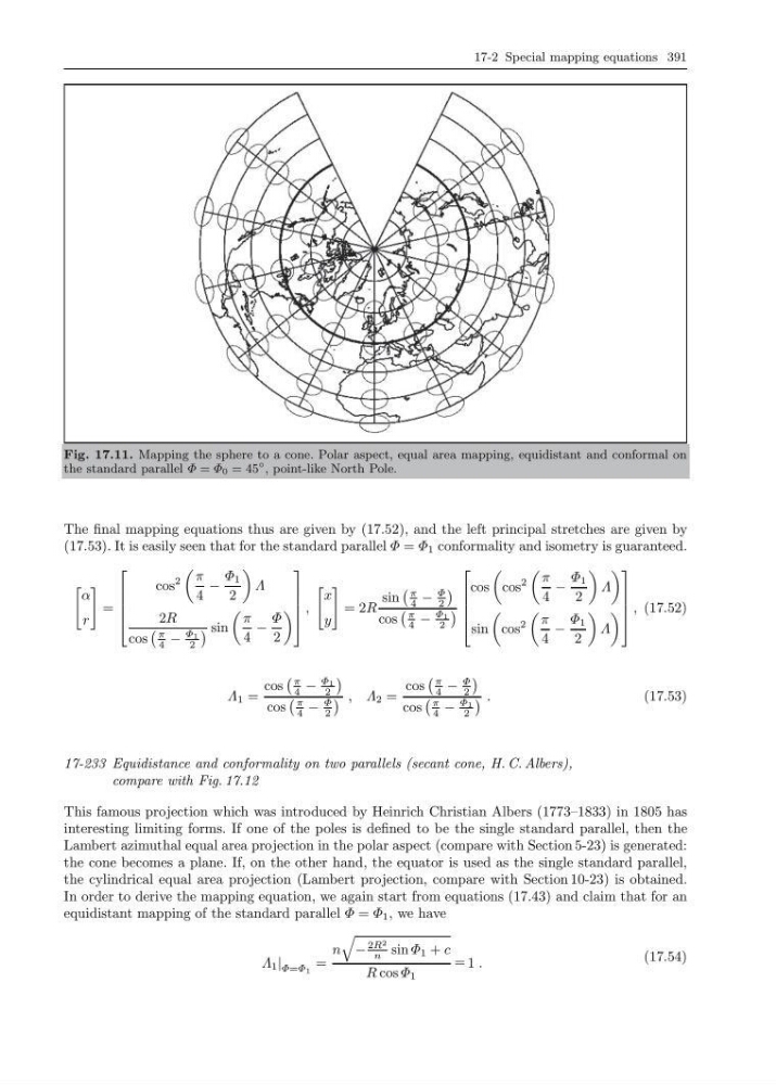
Fig. 17.11. Mapping the sphere to a cone. Polar aspect, equal area mapping, equidistant and conformal on
the standard parallel Φ = Φ 0 = 45
◦ , point-like North Pole.
The final mapping equations thus are given by (17.52), and the left principal stretches are given by
(17.53). It is easily seen that for the standard parallel Φ = Φ 1 conformality and isometry is guaranteed.
α
r
=
⎡
⎢
⎢
⎢
⎣
cos
2
π
4
−
Φ 1
2
Λ
2R
cos
π
4 −
Φ 1
2
sin
π
4
−
Φ
2
⎤
⎥
⎥
⎥
⎦
,
x
y
= 2R
sin
π
4 −
Φ
2
cos
π
4 −
Φ 1
2
⎡
⎢
⎢
⎢
⎣
cos
cos
2
π
4
−
Φ 1
2
Λ
sin
cos
2
π
4
−
Φ 1
2
Λ
⎤
⎥
⎥
⎥
⎦
, (17.52)
Λ 1 =
cos
π
4 −
Φ 1
2
cos
π
4 −
Φ
2
, Λ 2 =
cos
π
4 −
Φ
2
cos
π
4 −
Φ 1
2
.
(17.53)
17-233 Equidistance and conformality on two parallels (secant cone, H. C. Albers),
compare with Fig. 17.12
This famous projection which was introduced by Heinrich Christian Albers (1773–1833) in 1805 has
interesting limiting forms. If one of the poles is defined to be the single standard parallel, then the
Lambert azimuthal equal area projection in the polar aspect (compare with Section 5-23) is generated:
the cone becomes a plane. If, on the other hand, the equator is used as the single standard parallel,
the cylindrical equal area projection (Lambert projection, compare with Section 10-23) is obtained.
In order to derive the mapping equation, we again start from equations (17.43) and claim that for an
equidistant mapping of the standard parallel Φ = Φ 1 , we have
Λ 1 | Φ=Φ 1 =
n
−
2R 2
n sin Φ 1 + c
R cos Φ 1
= 1 .
(17.54)
Fig. 17.11. Mapping the sphere to a cone. Polar aspect, equal area mapping, equidistant and conformal on
the standard parallel Φ = Φ 0 = 45
◦ , point-like North Pole.
The final mapping equations thus are given by (17.52), and the left principal stretches are given by
(17.53). It is easily seen that for the standard parallel Φ = Φ 1 conformality and isometry is guaranteed.
α
r
=
⎡
⎢
⎢
⎢
⎣
cos
2
π
4
−
Φ 1
2
Λ
2R
cos
π
4 −
Φ 1
2
sin
π
4
−
Φ
2
⎤
⎥
⎥
⎥
⎦
,
x
y
= 2R
sin
π
4 −
Φ
2
cos
π
4 −
Φ 1
2
⎡
⎢
⎢
⎢
⎣
cos
cos
2
π
4
−
Φ 1
2
Λ
sin
cos
2
π
4
−
Φ 1
2
Λ
⎤
⎥
⎥
⎥
⎦
, (17.52)
Λ 1 =
cos
π
4 −
Φ 1
2
cos
π
4 −
Φ
2
, Λ 2 =
cos
π
4 −
Φ
2
cos
π
4 −
Φ 1
2
.
(17.53)
17-233 Equidistance and conformality on two parallels (secant cone, H. C. Albers),
compare with Fig. 17.12
This famous projection which was introduced by Heinrich Christian Albers (1773–1833) in 1805 has
interesting limiting forms. If one of the poles is defined to be the single standard parallel, then the
Lambert azimuthal equal area projection in the polar aspect (compare with Section 5-23) is generated:
the cone becomes a plane. If, on the other hand, the equator is used as the single standard parallel,
the cylindrical equal area projection (Lambert projection, compare with Section 10-23) is obtained.
In order to derive the mapping equation, we again start from equations (17.43) and claim that for an
equidistant mapping of the standard parallel Φ = Φ 1 , we have
Λ 1 | Φ=Φ 1 =
n
−
2R 2
n sin Φ 1 + c
R cos Φ 1
= 1 .
(17.54)