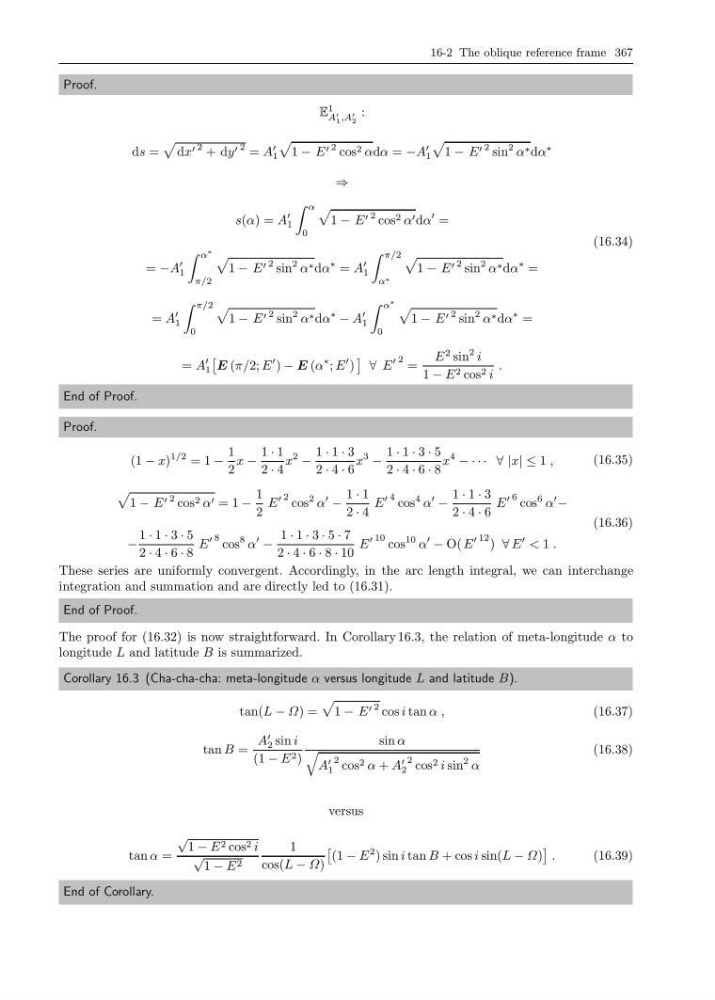
16-2 The oblique reference frame 367
Proof.
E
1
A
1 ,A
2
:
ds =
dx 2 + dy 2 = A
1
1 − E 2 cos 2 αdα = −A
1
1 − E 2 sin
2 α ∗ dα
∗
⇒
s(α) = A
1
α
0
1 − E 2 cos 2 α dα
=
= −A
1
α
∗
π/2
1 − E 2 sin
2 α ∗ dα
∗ = A
1
π/2
α ∗
1 − E 2 sin
2 α ∗ dα
∗ =
= A
1
π/2
0
1 − E 2 sin
2 α ∗ dα
∗
− A
1
α
∗
0
1 − E 2 sin
2 α ∗ dα
∗ =
= A
1
E (π/2; E
) − E (α
∗ ; E
)
∀ E
2 =
E
2 sin
2 i
1 − E 2 cos 2 i
.
(16.34)
End of Proof.
Proof.
(1 − x)
1/2 = 1 −
1
2
x −
1 · 1
2 · 4
x
2
−
1 · 1 · 3
2 · 4 · 6
x
3
−
1 · 1 · 3 · 5
2 · 4 · 6 · 8
x
4
− · · · ∀ |x| ≤ 1 ,
(16.35)
1 − E 2 cos 2 α = 1 −
1
2
E
2 cos
2 α
−
1 · 1
2 · 4
E
4 cos
4 α
−
1 · 1 · 3
2 · 4 · 6
E
6 cos
6 α
−
−
1 · 1 · 3 · 5
2 · 4 · 6 · 8
E
8 cos
8 α
−
1 · 1 · 3 · 5 · 7
2 · 4 · 6 · 8 · 10
E
10 cos
10 α
− O( E
12 ) ∀ E
< 1 .
(16.36)
These series are uniformly convergent. Accordingly, in the arc length integral, we can interchange
integration and summation and are directly led to (16.31).
End of Proof.
The proof for (16.32) is now straightforward. In Corollary 16.3, the relation of meta-longitude α to
longitude L and latitude B is summarized.
Corollary 16.3 (Cha-cha-cha: meta-longitude α versus longitude L and latitude B).
tan(L − Ω) =
1 − E 2 cos i tan α ,
(16.37)
tan B =
A
2 sin i
(1 − E 2 )
sin α
A
1
2 cos 2 α + A
2
2 cos 2 i sin
2 α
(16.38)
versus
tan α =
√
1 − E 2 cos 2 i
√
1 − E 2
1
cos(L − Ω)
(1 − E
2 ) sin i tan B + cos i sin(L − Ω)
.
(16.39)
End of Corollary.