

15-6 Strip transformation of conformal coordinates (Gauss–Krueger/UTM mappings) 351
15-612 The second step: polynomial representation of conformal coordinates in the second strip
replaced by the conformal coordinates in the first strip
The standard polynomial representation of conformal coordinates of type Gauss–Krueger or UTM
in the L 02 -strip is given by (15.117) and (15.118) subject to the longitude/latitude differences
l 2 := L − L 02 and b 2 := B − B 02 with respect to the longitude L 02 of the reference meridian and
the latitude B 02 of the reference point {L 02 , B 02 } of series expansion.
Easting: x 1 = ρ
x 10 l 2 + x 11 l 2 b 2 + x 30 l
3
2 + x 12 l 2 b
2
2 + O 4x
.
(15.117)
Northing: y 1 = ρ
y 0 + y 01 b 2 + y 20 l
2
2 + y 02 b
2
2 + y 21 l
2
2 b 2 + y 03 b
3
2 + O 4y
.
(15.118)
y 0 denotes the length of the meridian arc from zero ellipsoidal latitude to the ellipsoidal latitude B 02
of the reference point {L 02 , B 02 } chosen by the identity B 01 = B 02 = B 0 for operational reasons. The
coefficients {x ij , y ij } can be taken from Boxes 15.4 and 15.5. In addition, the optimal dilatation factor ρ
has been set identical in the L 01 -strip and the L 02 -strip of the same strip width. The longitude/latitude
differences {l 1 , b 1 } as well as {l 2 , b 2 } are related by l 2 = (L 01 −L 02 )+l 1 and b 2 = (B 01 −B 02 )+b 1 being
derived from the invariance L = L 01 + l 1 = L 02 + l 2 and B = B 01 + b 1 = B 02 + b 2 . Now we are on duty
to replace {l 2 , b 2 } by means of l 2 = (L 01 − L 02 ) + l 1 and b 2 = (B 01 − B 02 ) + b 1 by {(L 01 − L 02 ) + l 1 , b 1 }
within (15.117) and (15.118), which leads us to
x 2 = ρ
x 10 (L 01 − L 02 ) + x 10 l 1 + x 11 (L 01 − L 02 )b 1 + x 11 l 1 b 1 + x 30 (L 01 − L 02 )
3 +
+3x 30 (L 01 − L 02 )
2 l 1 + 3x 30 (L 01 − L 02 )l
2
1 + x 30 l
3
1 + x 12 (L 01 − L 02 )b
2
1 + x 12 l 1 b
2
1 + O 4x
,
(15.119)
y 2 = ρ
y 0 + y 01 b 1 + y 20 (L 01 − L 02 )
2 + 2y 20 (L 01 − L 02 )l 1 + y 20 l
2
1 + y 02 b
2
1 +
+y 21 (L 01 − L 02 )
2 b 1 + 2y 21 (L 01 − L 02 )l 1 b 1 + y 21 l
2
1 b 1 + y 03 b
3
1 + O 4y
.
(15.120)
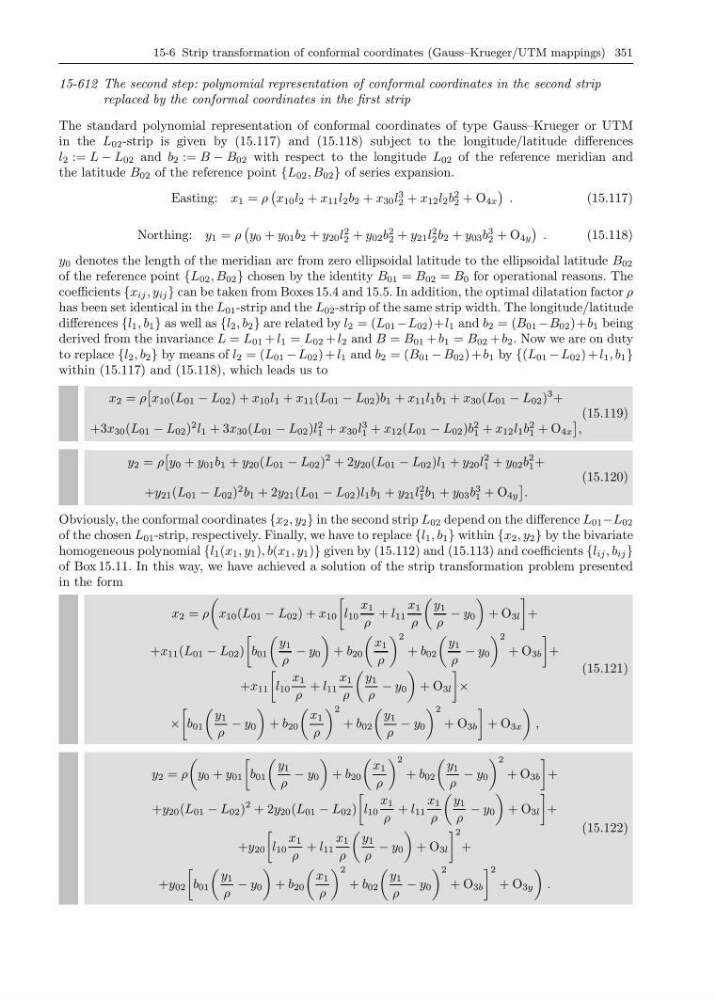
Obviously, the conformal coordinates {x 2 , y 2 } in the second strip L 02 depend on the difference L 01 −L 02
of the chosen L 01 -strip, respectively. Finally, we have to replace {l 1 , b 1 } within {x 2 , y 2 } by the bivariate
homogeneous polynomial {l 1 (x 1 , y 1 ), b(x 1 , y 1 )} given by (15.112) and (15.113) and coefficients {l ij , b ij }
of Box 15.11. In this way, we have achieved a solution of the strip transformation problem presented
in the form
x 2 = ρ
x 10 (L 01 − L 02 ) + x 10
l 10
x 1
ρ
+ l 11
x 1
ρ
y 1
ρ
− y 0
+ O 3l
+
+x 11 (L 01 − L 02 )
b 01
y 1
ρ
− y 0
+ b 20
x 1
ρ
2
+ b 02
y 1
ρ
− y 0
2
+ O 3b
+
+x 11
l 10
x 1
ρ
+ l 11
x 1
ρ
y 1
ρ
− y 0
+ O 3l
×
×
b 01
y 1
ρ
− y 0
+ b 20
x 1
ρ
2
+ b 02
y 1
ρ
− y 0
2
+ O 3b
+ O 3x
,
(15.121)
y 2 = ρ
y 0 + y 01
b 01
y 1
ρ
− y 0
+ b 20
x 1
ρ
2
+ b 02
y 1
ρ
− y 0
2
+ O 3b
+
+y 20 (L 01 − L 02 )
2 + 2y 20 (L 01 − L 02 )
l 10
x 1
ρ
+ l 11
x 1
ρ
y 1
ρ
− y 0
+ O 3l
+
+y 20
l 10
x 1
ρ
+ l 11
x 1
ρ
y 1
ρ
− y 0
+ O 3l
2
+
+y 02
b 01
y 1
ρ
− y 0
+ b 20
x 1
ρ
2
+ b 02
y 1
ρ
− y 0
2
+ O 3b
2
+ O 3y
.
(15.122)
15-612 The second step: polynomial representation of conformal coordinates in the second strip
replaced by the conformal coordinates in the first strip
The standard polynomial representation of conformal coordinates of type Gauss–Krueger or UTM
in the L 02 -strip is given by (15.117) and (15.118) subject to the longitude/latitude differences
l 2 := L − L 02 and b 2 := B − B 02 with respect to the longitude L 02 of the reference meridian and
the latitude B 02 of the reference point {L 02 , B 02 } of series expansion.
Easting: x 1 = ρ
x 10 l 2 + x 11 l 2 b 2 + x 30 l
3
2 + x 12 l 2 b
2
2 + O 4x
.
(15.117)
Northing: y 1 = ρ
y 0 + y 01 b 2 + y 20 l
2
2 + y 02 b
2
2 + y 21 l
2
2 b 2 + y 03 b
3
2 + O 4y
.
(15.118)
y 0 denotes the length of the meridian arc from zero ellipsoidal latitude to the ellipsoidal latitude B 02
of the reference point {L 02 , B 02 } chosen by the identity B 01 = B 02 = B 0 for operational reasons. The
coefficients {x ij , y ij } can be taken from Boxes 15.4 and 15.5. In addition, the optimal dilatation factor ρ
has been set identical in the L 01 -strip and the L 02 -strip of the same strip width. The longitude/latitude
differences {l 1 , b 1 } as well as {l 2 , b 2 } are related by l 2 = (L 01 −L 02 )+l 1 and b 2 = (B 01 −B 02 )+b 1 being
derived from the invariance L = L 01 + l 1 = L 02 + l 2 and B = B 01 + b 1 = B 02 + b 2 . Now we are on duty
to replace {l 2 , b 2 } by means of l 2 = (L 01 − L 02 ) + l 1 and b 2 = (B 01 − B 02 ) + b 1 by {(L 01 − L 02 ) + l 1 , b 1 }
within (15.117) and (15.118), which leads us to
x 2 = ρ
x 10 (L 01 − L 02 ) + x 10 l 1 + x 11 (L 01 − L 02 )b 1 + x 11 l 1 b 1 + x 30 (L 01 − L 02 )
3 +
+3x 30 (L 01 − L 02 )
2 l 1 + 3x 30 (L 01 − L 02 )l
2
1 + x 30 l
3
1 + x 12 (L 01 − L 02 )b
2
1 + x 12 l 1 b
2
1 + O 4x
,
(15.119)
y 2 = ρ
y 0 + y 01 b 1 + y 20 (L 01 − L 02 )
2 + 2y 20 (L 01 − L 02 )l 1 + y 20 l
2
1 + y 02 b
2
1 +
+y 21 (L 01 − L 02 )
2 b 1 + 2y 21 (L 01 − L 02 )l 1 b 1 + y 21 l
2
1 b 1 + y 03 b
3
1 + O 4y
.
(15.120)
Obviously, the conformal coordinates {x 2 , y 2 } in the second strip L 02 depend on the difference L 01 −L 02
of the chosen L 01 -strip, respectively. Finally, we have to replace {l 1 , b 1 } within {x 2 , y 2 } by the bivariate
homogeneous polynomial {l 1 (x 1 , y 1 ), b(x 1 , y 1 )} given by (15.112) and (15.113) and coefficients {l ij , b ij }
of Box 15.11. In this way, we have achieved a solution of the strip transformation problem presented
in the form
x 2 = ρ
x 10 (L 01 − L 02 ) + x 10
l 10
x 1
ρ
+ l 11
x 1
ρ
y 1
ρ
− y 0
+ O 3l
+
+x 11 (L 01 − L 02 )
b 01
y 1
ρ
− y 0
+ b 20
x 1
ρ
2
+ b 02
y 1
ρ
− y 0
2
+ O 3b
+
+x 11
l 10
x 1
ρ
+ l 11
x 1
ρ
y 1
ρ
− y 0
+ O 3l
×
×
b 01
y 1
ρ
− y 0
+ b 20
x 1
ρ
2
+ b 02
y 1
ρ
− y 0
2
+ O 3b
+ O 3x
,
(15.121)
y 2 = ρ
y 0 + y 01
b 01
y 1
ρ
− y 0
+ b 20
x 1
ρ
2
+ b 02
y 1
ρ
− y 0
2
+ O 3b
+
+y 20 (L 01 − L 02 )
2 + 2y 20 (L 01 − L 02 )
l 10
x 1
ρ
+ l 11
x 1
ρ
y 1
ρ
− y 0
+ O 3l
+
+y 20
l 10
x 1
ρ
+ l 11
x 1
ρ
y 1
ρ
− y 0
+ O 3l
2
+
+y 02
b 01
y 1
ρ
− y 0
+ b 20
x 1
ρ
2
+ b 02
y 1
ρ
− y 0
2
+ O 3b
2
+ O 3y
.
(15.122)