304 14 “Ellipsoid-of-revolution to cylinder”: polar aspect
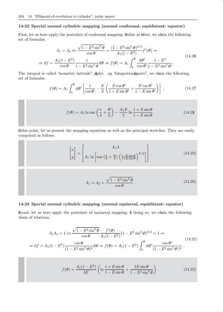
14-22 Special normal cylindric mapping (normal conformal, equidistant: equator)
First, let us here apply the postulate of conformal mapping. S
imilar as b efore, we ob tain the following
set of formulae.
Λ 1 = Λ 2 ⇔
1 − E 2 sin
2 Φ
cos Φ
=
(1 − E
2 sin
2 Φ)
3/2
A 1 (1 − E 2 )
f
(Φ) ⇒
⇒ df =
A 1 (1 − E
2 )
cos Φ
1
1 − E 2 sin
2 Φ
dΦ ⇒ f (Φ) = A 1
Φ
0
dΦ
cos Φ
1 − E
2
1 − E 2 sin
2 Φ .
(14.16 )
The integral is called “isometric latitude”. A pplyi ng “integration- b
y- parts”, we ob tain the following
set of formulae.
f (Φ) = A 1
Φ
0
dΦ
1
cos Φ −
E
2
E cos Φ
1 + E sin Φ +
E cos Φ
1 − E sin Φ
,
(14.17 )
f (Φ) = A 1 ln tan
π
4
+
Φ
2
−
A 1 E
2
ln
1 + E sin Φ
1 − E sin Φ
.
(14.18 )
A
t this point, let us present the mapping equations as well as the principal stretches. They are easily
computed as follows.
x
y
=
⎡
⎢
⎣
A 1 Λ
A 1 ln
tan
π
4 +
Φ
2
1−E sin Φ
1+E sin Φ
E/2
⎤
⎥
⎦ ,
(14.19)
Λ 1 = Λ 2 =
1 − E 2 sin
2 Φ
cos Φ
.
(14.20)
14-23 Special normal cylindric mapping (normal equiareal, equidistant: equator)
S econd, let us here apply the postulate of equiareal mapping. I
n doing so, we ob tain the following
chain of relations.
Λ 1 Λ 2 = 1 ⇔
1 − E 2 sin
2 Φ
cos Φ
f
(Φ)
A 1 (1 − E 2 )
(1 − E
2 sin
2 Φ)
3/2 = 1 ⇒
⇒ df = A 1 (1 − E
2 )
cos Φ
(1 − E 2 sin
2 Φ) 2 dΦ ⇒ f (Φ) = A 1 (1 − E
2 )
Φ
0
dΦ
cos Φ
(1 − E 2 sin
2 Φ ) 2 ,
(14.21)
f (Φ) =
A 1 (1 − E
2 )
4E
ln
1 + E sin Φ
1 − E sin Φ
+
2E sin Φ
1 − E 2 sin
2 Φ
.
(14.22)