

252 8 “Ellipsoid-of-revolution to tangential plane”
P c
n = G 3
P 0
p
r = p − P 0
h = H 0
˙
X P − X c
˛
˛ − n
¸
X P − X c
X P − X c −
˙
X P − X c
˛
˛ n
¸
n
P
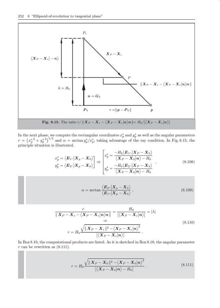
Fig. 8.15. The ratio r/ X P − X c −
˙
X P − X c
˛
˛ n
¸
n = H 0 /
˛
˛
˙
X P − X c
˛
˛ n
¸˛
˛ .
In the next phase, we compute the rectangular coordinates x
∗
p and y
∗
p as well as the angular parameters
r =
x
∗
p
2 + y
∗
p
2
1/2 and α = arctan y
∗
p /x
∗
p , taking advantage of the ray condition. In Fig. 8.15, the
principle situation is illustrated.
x
∗
p =
E 1 ∗
X p − X 0
y
∗
p =
E 2 ∗
X p − X 0
⇒
⎡
⎢
⎢
⎢
⎢
⎣
x
∗
p =
−H 0
E 1 ∗
X P − X 0
X P − X 0
n
− H 0
y
∗
p =
−H 0
E 2 ∗
X P − X 0
X P − X 0
n
− H 0
,
(8.108)
α = arctan
E 2 ∗
X p − X 0
E 1 ∗
X p − X 0
,
(8.109)
r
X P − X c −
X P − X c
n
n
=
H 0
X P − X c
n
= |λ|
⇒
r = H 0
X P − X c 2 −
X P − X c
n
2
X P − X c
n
.
(8.110)
In Box 8.10, the computational products are listed. As it is sketched in Box 8.10, the angular parameter
r can be rewritten as (8.111).
r = H 0
X P − X 0 2 −
X P − X 0
n
2
X P − X 0
n
− H 0
.
(8.111)
P c
n = G 3
P 0
p
r = p − P 0
h = H 0
˙
X P − X c
˛
˛ − n
¸
X P − X c
X P − X c −
˙
X P − X c
˛
˛ n
¸
n
P
Fig. 8.15. The ratio r/ X P − X c −
˙
X P − X c
˛
˛ n
¸
n = H 0 /
˛
˛
˙
X P − X c
˛
˛ n
¸˛
˛ .
In the next phase, we compute the rectangular coordinates x
∗
p and y
∗
p as well as the angular parameters
r =
x
∗
p
2 + y
∗
p
2
1/2 and α = arctan y
∗
p /x
∗
p , taking advantage of the ray condition. In Fig. 8.15, the
principle situation is illustrated.
x
∗
p =
E 1 ∗
X p − X 0
y
∗
p =
E 2 ∗
X p − X 0
⇒
⎡
⎢
⎢
⎢
⎢
⎣
x
∗
p =
−H 0
E 1 ∗
X P − X 0
X P − X 0
n
− H 0
y
∗
p =
−H 0
E 2 ∗
X P − X 0
X P − X 0
n
− H 0
,
(8.108)
α = arctan
E 2 ∗
X p − X 0
E 1 ∗
X p − X 0
,
(8.109)
r
X P − X c −
X P − X c
n
n
=
H 0
X P − X c
n
= |λ|
⇒
r = H 0
X P − X c 2 −
X P − X c
n
2
X P − X c
n
.
(8.110)
In Box 8.10, the computational products are listed. As it is sketched in Box 8.10, the angular parameter
r can be rewritten as (8.111).
r = H 0
X P − X 0 2 −
X P − X 0
n
2
X P − X 0
n
− H 0
.
(8.111)