

238 8 “Ellipsoid-of-revolution to tangential plane”
8-23 Equiareal mapping
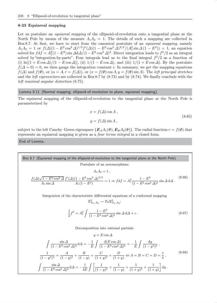
Let us postulate an equiareal mapping of the ellipsoid-of-revolution onto a tangential plane at the
North Pole by means of the measure Λ 1 Λ 2 = 1. The details of such a mapping are collected in
Box 8.7. At first, we have to start from the canonical postulate of an equiareal mapping, namely
Λ 1 Λ 2 = 1 or f (∆)(1 − E
2 cos
2 ∆)
1/2 f
(∆)(1 − E
2 cos
2 ∆)
3/2 /(A
2
1 sin ∆ (1 − E
2 )) = 1, an equation
solved for f df = A
2
1 (1 − E
2 ) sin ∆d∆/(1 − E
2 cos
2 ∆)
2 . Direct integration leads to f
2 /2 as an integral
solved by“integration-by-parts”. Four integrals lead us to the final integral f
2 /2 as a function of
(i) ln[(1 + E cos ∆)/(1 − E cos ∆)], (ii) 1/(1 − E cos ∆), and (iii) 1/(1 + E cos ∆). By the postulate
f (∆ = 0) = 0, we then gauge the integration constant c. In summary, we get the mapping equations
f (∆) and f (Φ), or (α = A, r = f (∆)), or (x = f (Φ) cos Λ, y = f (Φ) sin Λ). The left principal stretches
and the left eigenvectors are collected in Box 8.7 by (8.73) and by (8.74). We finally conclude with the
left maximal angular distortion (8.75).
Lemma 8.11 (Normal mapping: ellipsoid-of-revolution to plane, equiareal mapping).
The equiareal mapping of the ellipsoid-of-revolution to the tangential plane at the North Pole is
parameterized by
x = f (∆) cos Λ ,
y = f (∆) sin Λ ,
(8.65)
subject to the left Cauchy–Green eigenspace {E Λ Λ 1 (Φ), E Φ Λ 2 (Φ)}. The radial function r = f (Φ) that
represents an equiareal mapping is given as a four terms integral in a closed form.
End of Lemma.
Box 8.7 (Equiareal mapping of the ellipsoid-of-revolution to the tangential plane at the North Pole).
Postulate of an areomorphism:
Λ 1 Λ 2 = 1 ,
f (∆)
√
1 − E 2 cos 2 ∆
A 1 sin ∆
f
(∆)(1 − E
2 cos
2 ∆)
3/2
A 1 (1 − E 2 )
= 1 ⇒ f df = A
2
1
1 − E
2
(1 − E 2 cos 2 ∆) 2 sin ∆ d∆ .
(8.66)
Integration of the characteristic differential equations of a conformal mapping
E
2
A 1 ,A 2 → T N E
2
A 1 ,A 2 :
1
2
f
2 = A
2
1
Z
1 − E
2
(1 − E 2 cos 2 ∆) 2 sin ∆ d∆ + c .
(8.67)
Decomposition into rational partials:
y = E cos ∆
Z
sin ∆
(1 − E 2 cos 2 ∆) 2 d∆ = −
1
E
Z
d(E cos ∆)
(1 − E 2 cos 2 ∆) 2 = −
1
E
Z
dy
(1 − y 2 ) 2 ,
1
(1 − y 2 ) 2 =
A
(1 − y) 2 +
B
(1 − y)
+
C
(1 + y) 2 +
D
(1 + y)
⇔ A = B = C = D =
1
4
,
Z
sin ∆
(1 − E 2 cos 2 ∆) 2 d∆ = −
1
4E
Z »
1
(1 − y) 2 +
1
(1 − y)
+
1
(1 + y) 2 +
1
(1 + y)
–
dy .
(8.68)
8-23 Equiareal mapping
Let us postulate an equiareal mapping of the ellipsoid-of-revolution onto a tangential plane at the
North Pole by means of the measure Λ 1 Λ 2 = 1. The details of such a mapping are collected in
Box 8.7. At first, we have to start from the canonical postulate of an equiareal mapping, namely
Λ 1 Λ 2 = 1 or f (∆)(1 − E
2 cos
2 ∆)
1/2 f
(∆)(1 − E
2 cos
2 ∆)
3/2 /(A
2
1 sin ∆ (1 − E
2 )) = 1, an equation
solved for f df = A
2
1 (1 − E
2 ) sin ∆d∆/(1 − E
2 cos
2 ∆)
2 . Direct integration leads to f
2 /2 as an integral
solved by“integration-by-parts”. Four integrals lead us to the final integral f
2 /2 as a function of
(i) ln[(1 + E cos ∆)/(1 − E cos ∆)], (ii) 1/(1 − E cos ∆), and (iii) 1/(1 + E cos ∆). By the postulate
f (∆ = 0) = 0, we then gauge the integration constant c. In summary, we get the mapping equations
f (∆) and f (Φ), or (α = A, r = f (∆)), or (x = f (Φ) cos Λ, y = f (Φ) sin Λ). The left principal stretches
and the left eigenvectors are collected in Box 8.7 by (8.73) and by (8.74). We finally conclude with the
left maximal angular distortion (8.75).
Lemma 8.11 (Normal mapping: ellipsoid-of-revolution to plane, equiareal mapping).
The equiareal mapping of the ellipsoid-of-revolution to the tangential plane at the North Pole is
parameterized by
x = f (∆) cos Λ ,
y = f (∆) sin Λ ,
(8.65)
subject to the left Cauchy–Green eigenspace {E Λ Λ 1 (Φ), E Φ Λ 2 (Φ)}. The radial function r = f (Φ) that
represents an equiareal mapping is given as a four terms integral in a closed form.
End of Lemma.
Box 8.7 (Equiareal mapping of the ellipsoid-of-revolution to the tangential plane at the North Pole).
Postulate of an areomorphism:
Λ 1 Λ 2 = 1 ,
f (∆)
√
1 − E 2 cos 2 ∆
A 1 sin ∆
f
(∆)(1 − E
2 cos
2 ∆)
3/2
A 1 (1 − E 2 )
= 1 ⇒ f df = A
2
1
1 − E
2
(1 − E 2 cos 2 ∆) 2 sin ∆ d∆ .
(8.66)
Integration of the characteristic differential equations of a conformal mapping
E
2
A 1 ,A 2 → T N E
2
A 1 ,A 2 :
1
2
f
2 = A
2
1
Z
1 − E
2
(1 − E 2 cos 2 ∆) 2 sin ∆ d∆ + c .
(8.67)
Decomposition into rational partials:
y = E cos ∆
Z
sin ∆
(1 − E 2 cos 2 ∆) 2 d∆ = −
1
E
Z
d(E cos ∆)
(1 − E 2 cos 2 ∆) 2 = −
1
E
Z
dy
(1 − y 2 ) 2 ,
1
(1 − y 2 ) 2 =
A
(1 − y) 2 +
B
(1 − y)
+
C
(1 + y) 2 +
D
(1 + y)
⇔ A = B = C = D =
1
4
,
Z
sin ∆
(1 − E 2 cos 2 ∆) 2 d∆ = −
1
4E
Z »
1
(1 − y) 2 +
1
(1 − y)
+
1
(1 + y) 2 +
1
(1 + y)
–
dy .
(8.68)