

2-2 Eigenspace analysis, Euler–Lagrange deformation tensor 99
Ex ample 2.1(O rthogonal proj ection of points of the sphere
S
2
R + onto the equatorial plane P
2
O through
the origin O).
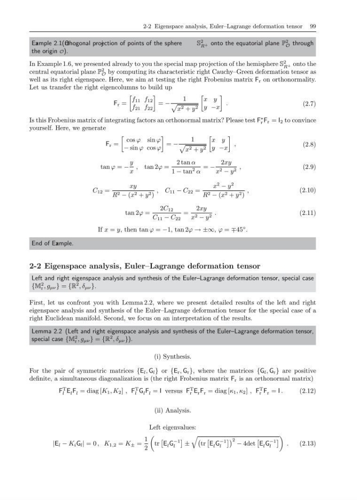
In Example 1.6, we presented already to you the special map projection of the hemisphere S
2
R + onto the
central equatorial plane P
2
O by computing its characteristic right Cauchy–Green deformation tensor as
well as its right eigenspace. Here, we aim at testing the right Frobenius matrix F r on orthonormality.
Let us transfer the right eigencolumns to build up
F r =
f 11 f 12
f 21 f 22
= −
1
x 2 + y 2
x y
y −x
.
(2.7)
Is this Frobenius matrix of integrating factors an orthonormal matrix? Please test F
∗
r F r = I 2 to convince
yourself. Here, we generate
F r =
cos ϕ sin ϕ
− sin ϕ cos ϕ
= −
1
x 2 + y 2
x y
y −x
,
(2.8)
tan ϕ = −
y
x
, tan 2ϕ =
2 tan α
1 − tan
2 α
= −
2xy
x 2 − y 2 ,
(2.9)
C 12 =
xy
R 2 − (x 2 + y 2 )
, C 11 − C 22 =
x
2
− y
2
R 2 − (x 2 + y 2 )
,
(2.10)
tan 2ϕ =
2C 12
C 11 − C 22
=
2xy
x 2 − y 2 .
(2.11)
If x = y, then tan ϕ = −1, tan 2ϕ → ±∞, ϕ = ∓45
◦ .
End of Ex ample.
2-2 Eigenspace analysis, Euler–Lagrange deformation tensor
Left and right eigenspace analysis and synthesis of the Euler–Lagrange deformation tensor, special case
{M
2
r , g µν } = {R
2 , δ µν }.
First, let us confront you with Lemma 2.2, where we present detailed results of the left and right
eigenspace analysis and synthesis of the Euler–Lagrange deformation tensor for the special case of a
right Euclidean manifold. Second, we focus on an interpretation of the results.
Lemma 2.2 (Left and right eigenspace analysis and synthesis of the Euler–Lagrange deformation tensor,
special case {M
2
r , g µν } = {R
2 , δ µν }).
(i) Synthesis.
For the pair of symmetric matrices {E l , G l } or {E r , G r }, where the matrices {G l , G r } are positive
definite, a simultaneous diagonalization is (the right Frobenius matrix F r is an orthonormal matrix)
F
T
l E l F l = diag [K 1 , K 2 ] , F
T
l G l F l = I versus F
T
r E r F r = diag [κ 1 , κ 2 ] , F
T
r F r = I .
(2.12)
(ii) Analysis.
Left eigenvalues:
|E l − K i G l | = 0 , K 1,2 = K ± =
1
2
tr
E l G
−1
l
±
tr
E l G
−1
l
2 − 4det
E l G
−1
l
.
(2.13)
Ex ample 2.1(O rthogonal proj ection of points of the sphere
S
2
R + onto the equatorial plane P
2
O through
the origin O).
In Example 1.6, we presented already to you the special map projection of the hemisphere S
2
R + onto the
central equatorial plane P
2
O by computing its characteristic right Cauchy–Green deformation tensor as
well as its right eigenspace. Here, we aim at testing the right Frobenius matrix F r on orthonormality.
Let us transfer the right eigencolumns to build up
F r =
f 11 f 12
f 21 f 22
= −
1
x 2 + y 2
x y
y −x
.
(2.7)
Is this Frobenius matrix of integrating factors an orthonormal matrix? Please test F
∗
r F r = I 2 to convince
yourself. Here, we generate
F r =
cos ϕ sin ϕ
− sin ϕ cos ϕ
= −
1
x 2 + y 2
x y
y −x
,
(2.8)
tan ϕ = −
y
x
, tan 2ϕ =
2 tan α
1 − tan
2 α
= −
2xy
x 2 − y 2 ,
(2.9)
C 12 =
xy
R 2 − (x 2 + y 2 )
, C 11 − C 22 =
x
2
− y
2
R 2 − (x 2 + y 2 )
,
(2.10)
tan 2ϕ =
2C 12
C 11 − C 22
=
2xy
x 2 − y 2 .
(2.11)
If x = y, then tan ϕ = −1, tan 2ϕ → ±∞, ϕ = ∓45
◦ .
End of Ex ample.
2-2 Eigenspace analysis, Euler–Lagrange deformation tensor
Left and right eigenspace analysis and synthesis of the Euler–Lagrange deformation tensor, special case
{M
2
r , g µν } = {R
2 , δ µν }.
First, let us confront you with Lemma 2.2, where we present detailed results of the left and right
eigenspace analysis and synthesis of the Euler–Lagrange deformation tensor for the special case of a
right Euclidean manifold. Second, we focus on an interpretation of the results.
Lemma 2.2 (Left and right eigenspace analysis and synthesis of the Euler–Lagrange deformation tensor,
special case {M
2
r , g µν } = {R
2 , δ µν }).
(i) Synthesis.
For the pair of symmetric matrices {E l , G l } or {E r , G r }, where the matrices {G l , G r } are positive
definite, a simultaneous diagonalization is (the right Frobenius matrix F r is an orthonormal matrix)
F
T
l E l F l = diag [K 1 , K 2 ] , F
T
l G l F l = I versus F
T
r E r F r = diag [κ 1 , κ 2 ] , F
T
r F r = I .
(2.12)
(ii) Analysis.
Left eigenvalues:
|E l − K i G l | = 0 , K 1,2 = K ± =
1
2
tr
E l G
−1
l
±
tr
E l G
−1
l
2 − 4det
E l G
−1
l
.
(2.13)