

98
2 From Riemann manifolds to Euclidean manifolds
Left eigencolumns:
F 11
F 21
=
1
G 11 (c 22 − Λ 2
1 G 22 ) 2 − 2G 12 (c 12 − Λ 2
1 G 12 )(c 22 − Λ 2
1 G 22 ) + G 22 (c 12 − Λ 2
1 G 12 ) 2
×
×
+(c 22 − Λ
2
1 G 22 )
−(c 12 − Λ
2
1 G 12 )
,
F 12
F 22
=
1
G 22 (c 11 − Λ 2
2 G 11 ) 2 − 2G 12 (c 11 − Λ 2
2 G 11 )(c 12 − Λ 2
2 G 12 ) + G 11 (c 12 − Λ 2
2 G 12 ) 2
×
×
−(c 12 − Λ
2
2 G 12 )
+(c 11 − Λ
2
2 G 11 )
.
(2.3)
Right eigenvalues or right principal stretches
(the right general eigenvalue problem reduces to the right special eigenvalue problem):
C r − λ
2
i G r
= |C r − λ i I 2 | = 0 ∀ i ∈ {1, 2} ,
λ
2
1,2 = λ
2
± =
1
2
tr
C r G
−1
r
±
tr
C r G
−1
r
2 − 4det
C r G
−1
r
=
=
1
2
C 11 + C 22 ±
(C 11 − C 22 ) 2 + (2C 12 ) 2
.
(2.4)
Right eigencolumns:
F r =
f 11 f 12
f 21 f 22
⎧
⎪ ⎪ ⎪ ⎪ ⎨
⎪ ⎪ ⎪ ⎪ ⎩
f 11
f 21
=
1
(C 22 − λ 2
1 ) 2 + C 2
12
C 22 − λ
2
1
−C 12
,
f 12
f 22
=
1
(C 11 − λ 2
2 ) 2 + C 2
12
−C 12
C 11 − λ
2
2
.
(2.5)
Since the right Frobenius matrix F r is an orthonormal matrix, it can be represented by
F r =
cos ϕ sin ϕ
− sin ϕ cos ϕ
∀ ϕ ∈ [0, 2π] ,
tan ϕ =
C 12
C 11 − λ 2
−
, tan 2ϕ =
2C 12
C 11 − C 22
.
(2.6)
End of Lemma.
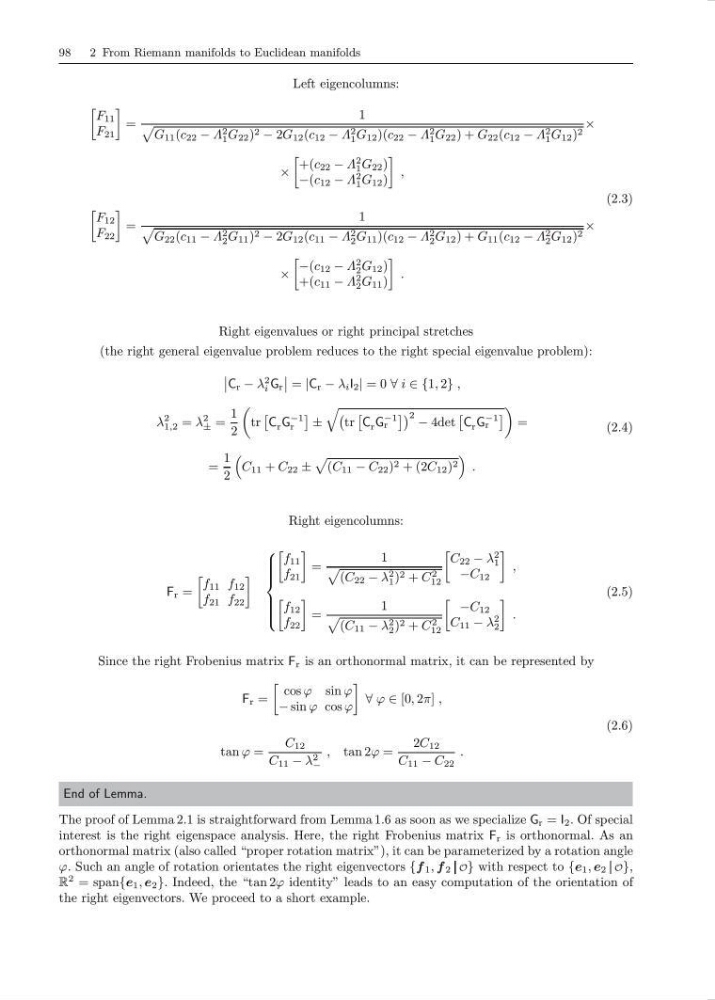
The proof of Lemma 2.1 is straightforward from Lemma 1.6 as soon as we specialize G r = I 2 . Of special
interest is the right eigenspace analysis. Here, the right Frobenius matrix F r is orthonormal. As an
orthonormal matrix (also called “proper rotation matrix”), it can be parameterized by a rotation angle
ϕ. Such an angle of rotation orientates the right eigenvectors {f 1 , f 2 O} with respect to {e 1 , e 2 O},
R
2 = span{e 1 , e 2 }. Indeed, the “tan 2ϕ identity” leads to an easy computation of the orientation of
the right eigenvectors. We proceed to a short example.
2 From Riemann manifolds to Euclidean manifolds
Left eigencolumns:
F 11
F 21
=
1
G 11 (c 22 − Λ 2
1 G 22 ) 2 − 2G 12 (c 12 − Λ 2
1 G 12 )(c 22 − Λ 2
1 G 22 ) + G 22 (c 12 − Λ 2
1 G 12 ) 2
×
×
+(c 22 − Λ
2
1 G 22 )
−(c 12 − Λ
2
1 G 12 )
,
F 12
F 22
=
1
G 22 (c 11 − Λ 2
2 G 11 ) 2 − 2G 12 (c 11 − Λ 2
2 G 11 )(c 12 − Λ 2
2 G 12 ) + G 11 (c 12 − Λ 2
2 G 12 ) 2
×
×
−(c 12 − Λ
2
2 G 12 )
+(c 11 − Λ
2
2 G 11 )
.
(2.3)
Right eigenvalues or right principal stretches
(the right general eigenvalue problem reduces to the right special eigenvalue problem):
C r − λ
2
i G r
= |C r − λ i I 2 | = 0 ∀ i ∈ {1, 2} ,
λ
2
1,2 = λ
2
± =
1
2
tr
C r G
−1
r
±
tr
C r G
−1
r
2 − 4det
C r G
−1
r
=
=
1
2
C 11 + C 22 ±
(C 11 − C 22 ) 2 + (2C 12 ) 2
.
(2.4)
Right eigencolumns:
F r =
f 11 f 12
f 21 f 22
⎧
⎪ ⎪ ⎪ ⎪ ⎨
⎪ ⎪ ⎪ ⎪ ⎩
f 11
f 21
=
1
(C 22 − λ 2
1 ) 2 + C 2
12
C 22 − λ
2
1
−C 12
,
f 12
f 22
=
1
(C 11 − λ 2
2 ) 2 + C 2
12
−C 12
C 11 − λ
2
2
.
(2.5)
Since the right Frobenius matrix F r is an orthonormal matrix, it can be represented by
F r =
cos ϕ sin ϕ
− sin ϕ cos ϕ
∀ ϕ ∈ [0, 2π] ,
tan ϕ =
C 12
C 11 − λ 2
−
, tan 2ϕ =
2C 12
C 11 − C 22
.
(2.6)
End of Lemma.
The proof of Lemma 2.1 is straightforward from Lemma 1.6 as soon as we specialize G r = I 2 . Of special
interest is the right eigenspace analysis. Here, the right Frobenius matrix F r is orthonormal. As an
orthonormal matrix (also called “proper rotation matrix”), it can be parameterized by a rotation angle
ϕ. Such an angle of rotation orientates the right eigenvectors {f 1 , f 2 O} with respect to {e 1 , e 2 O},
R
2 = span{e 1 , e 2 }. Indeed, the “tan 2ϕ identity” leads to an easy computation of the orientation of
the right eigenvectors. We proceed to a short example.