

88
1 From Riemann manifolds to Riemann manifolds
Box 1.53 (Reference frames (3-leg) of type Gauss, Cartan, and Darboux).
The left manifolds (M
1
l ⊂ M
2
l , G 12 = 0).
Gauss:
Cartan:
Darboux:
G 1 :=
∂X (U, V )
∂U
,
C 1 :=
G 1
G 1
=
G 1
√
G 11
,
D 1 := X
=
dX
dS
,
G 2 :=
∂X (U, V )
∂V
,
C 2 :=
G 2
G 2
=
G 2
√
G 22
,
D 2 := D 3 ×D 1 =
= ∗ (D 3 ∧ D 1 ) ,
G 3 :=
G 1 ×G 2
G 1 ×G 2
.
C 3 := C 1 ×C 2 =
= ∗ (C 1 ∧ C 2 ) = G 3 .
D 3 = C 3 = G 3 .
(1.322)
The right manifolds (c 12 = 0).
Gauss:
Cartan:
Darboux:
g 1 :=
∂x
`
u(U ), v(V )
´
∂U
,
c 1 :=
g 1
g 1
,
d 1 := x
=
dx
`
u(s), v(s)
´
ds
,
g 2 :=
∂x
`
u(U ), v(V )
´
∂V
,
c 2 :=
g 2
g 2
,
d 2 := d 3 ×d 1 =
= ∗ (d 3 ∧ d 1 ) ,
g 3 :=
g 1 ×g 2
g 1 ×g 2
.
c 3 := c 1 ×c 2 =
= ∗ (c 1 ∧ c 2 ) .
d 3 = c 3 = g 3 .
(1.323)
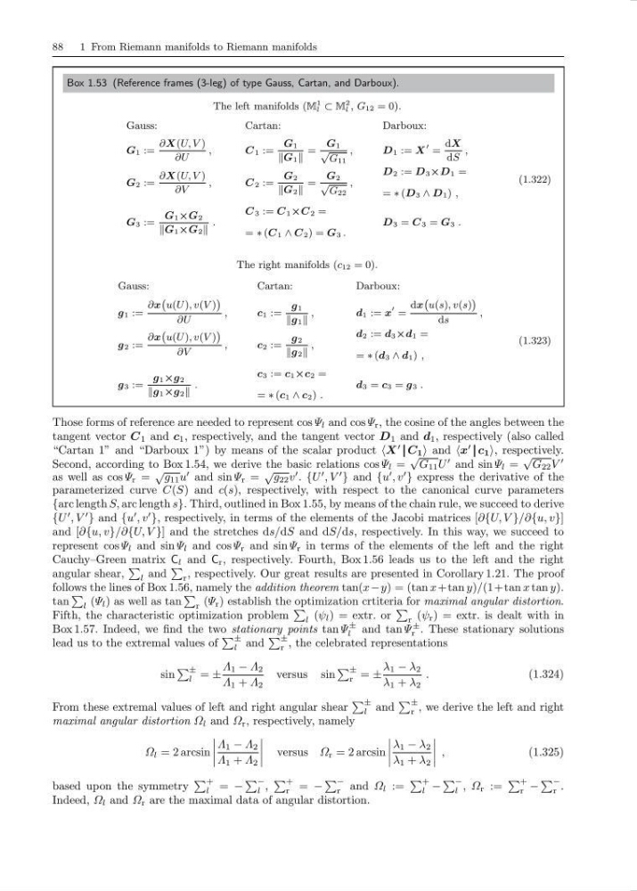
Those forms of reference are needed to represent cos Ψ l and cos Ψ r , the cosine of the angles between the
tangent vector C 1 and c 1 , respectively, and the tangent vector D 1 and d 1 , respectively (also called
“Cartan 1” and “Darboux 1”) by means of the scalar product X
C 1 and x
c 1 , respectively.
Second, according to Box 1.54, we derive the basic relations cos Ψ l =
√
G 11 U
and sin Ψ l =
√
G 22 V
as well as cos Ψ r =
√ g 11 u
and sin Ψ r =
√
g 22 v
. {U
, V
} and {u
, v
} express the derivative of the
parameterized curve C(S) and c(s), respectively, with respect to the canonical curve parameters
{arc length S, arc length s}. Third, outlined in Box 1.55, by means of the chain rule, we succeed to derive
{U
, V
} and {u
, v
}, respectively, in terms of the elements of the Jacobi matrices [∂{U, V }/∂{u, v}]
and [∂{u, v}/∂{U, V }] and the stretches ds/dS and dS/ds, respectively. In this way, we succeed to
represent cos Ψ l and sin Ψ l and cos Ψ r and sin Ψ r in terms of the elements of the left and the right
Cauchy–Green matrix C l and C r , respectively. Fourth, Box 1.56 leads us to the left and the right
angular shear,
l and
r , respectively. Our great results are presented in Corollary 1.21. The proof
follows the lines of Box 1.56, namely the addition theorem tan(x−y) = (tan x+tan y)/(1+tan x tan y).
tan
l (Ψ l ) as well as tan
r (Ψ r ) establish the optimization crtiteria for maximal angular distortion.
Fifth, the characteristic optimization problem
l (ψ l ) = extr. or
r (ψ r ) = extr. is dealt with in
Box 1.57. Indeed, we find the two stationary points tan Ψ
±
l and tan Ψ
±
r . These stationary solutions
lead us to the extremal values of
±
l and
±
r , the celebrated representations
sin
±
l = ±
Λ 1 − Λ 2
Λ 1 + Λ 2
versus sin
±
r = ±
λ 1 − λ 2
λ 1 + λ 2
.
(1.324)
From these extremal values of left and right angular shear
±
l and
±
r , we derive the left and right
maximal angular distortion Ω l and Ω r , respectively, namely
Ω l = 2 arcsin
Λ 1 − Λ 2
Λ 1 + Λ 2
versus Ω r = 2 arcsin
λ 1 − λ 2
λ 1 + λ 2
,
(1.325)
based upon the symmetry
+
l = −
−
l ,
+
r = −
−
r and Ω l :=
+
l −
−
l , Ω r :=
+
r −
−
r .
Indeed, Ω l and Ω r are the maximal data of angular distortion.
1 From Riemann manifolds to Riemann manifolds
Box 1.53 (Reference frames (3-leg) of type Gauss, Cartan, and Darboux).
The left manifolds (M
1
l ⊂ M
2
l , G 12 = 0).
Gauss:
Cartan:
Darboux:
G 1 :=
∂X (U, V )
∂U
,
C 1 :=
G 1
G 1
=
G 1
√
G 11
,
D 1 := X
=
dX
dS
,
G 2 :=
∂X (U, V )
∂V
,
C 2 :=
G 2
G 2
=
G 2
√
G 22
,
D 2 := D 3 ×D 1 =
= ∗ (D 3 ∧ D 1 ) ,
G 3 :=
G 1 ×G 2
G 1 ×G 2
.
C 3 := C 1 ×C 2 =
= ∗ (C 1 ∧ C 2 ) = G 3 .
D 3 = C 3 = G 3 .
(1.322)
The right manifolds (c 12 = 0).
Gauss:
Cartan:
Darboux:
g 1 :=
∂x
`
u(U ), v(V )
´
∂U
,
c 1 :=
g 1
g 1
,
d 1 := x
=
dx
`
u(s), v(s)
´
ds
,
g 2 :=
∂x
`
u(U ), v(V )
´
∂V
,
c 2 :=
g 2
g 2
,
d 2 := d 3 ×d 1 =
= ∗ (d 3 ∧ d 1 ) ,
g 3 :=
g 1 ×g 2
g 1 ×g 2
.
c 3 := c 1 ×c 2 =
= ∗ (c 1 ∧ c 2 ) .
d 3 = c 3 = g 3 .
(1.323)
Those forms of reference are needed to represent cos Ψ l and cos Ψ r , the cosine of the angles between the
tangent vector C 1 and c 1 , respectively, and the tangent vector D 1 and d 1 , respectively (also called
“Cartan 1” and “Darboux 1”) by means of the scalar product X
C 1 and x
c 1 , respectively.
Second, according to Box 1.54, we derive the basic relations cos Ψ l =
√
G 11 U
and sin Ψ l =
√
G 22 V
as well as cos Ψ r =
√ g 11 u
and sin Ψ r =
√
g 22 v
. {U
, V
} and {u
, v
} express the derivative of the
parameterized curve C(S) and c(s), respectively, with respect to the canonical curve parameters
{arc length S, arc length s}. Third, outlined in Box 1.55, by means of the chain rule, we succeed to derive
{U
, V
} and {u
, v
}, respectively, in terms of the elements of the Jacobi matrices [∂{U, V }/∂{u, v}]
and [∂{u, v}/∂{U, V }] and the stretches ds/dS and dS/ds, respectively. In this way, we succeed to
represent cos Ψ l and sin Ψ l and cos Ψ r and sin Ψ r in terms of the elements of the left and the right
Cauchy–Green matrix C l and C r , respectively. Fourth, Box 1.56 leads us to the left and the right
angular shear,
l and
r , respectively. Our great results are presented in Corollary 1.21. The proof
follows the lines of Box 1.56, namely the addition theorem tan(x−y) = (tan x+tan y)/(1+tan x tan y).
tan
l (Ψ l ) as well as tan
r (Ψ r ) establish the optimization crtiteria for maximal angular distortion.
Fifth, the characteristic optimization problem
l (ψ l ) = extr. or
r (ψ r ) = extr. is dealt with in
Box 1.57. Indeed, we find the two stationary points tan Ψ
±
l and tan Ψ
±
r . These stationary solutions
lead us to the extremal values of
±
l and
±
r , the celebrated representations
sin
±
l = ±
Λ 1 − Λ 2
Λ 1 + Λ 2
versus sin
±
r = ±
λ 1 − λ 2
λ 1 + λ 2
.
(1.324)
From these extremal values of left and right angular shear
±
l and
±
r , we derive the left and right
maximal angular distortion Ω l and Ω r , respectively, namely
Ω l = 2 arcsin
Λ 1 − Λ 2
Λ 1 + Λ 2
versus Ω r = 2 arcsin
λ 1 − λ 2
λ 1 + λ 2
,
(1.325)
based upon the symmetry
+
l = −
−
l ,
+
r = −
−
r and Ω l :=
+
l −
−
l , Ω r :=
+
r −
−
r .
Indeed, Ω l and Ω r are the maximal data of angular distortion.