

3.2. Some Canonical Problems Having Analytic Solutions
57
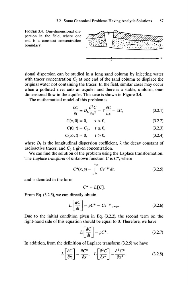
FIGURE 3.4. One-dimensional dispersion in the field, where one
end is a constant concentration
boundary.
o
.. x
sional dispersion can be studied in a long sand column by injecting water
with tracer concentration Co at one end of the sand column to displace the
original water not containing the tracer. In the field, similar cases may occur
when apolluted river cuts an aquifer and there is a stable, uniform, onedimensional flow in the aquifer. This case is shown in Figure 3.4.
The mathematical model of this problem is
oC
02C
oC
at = DL ox2 - V ox - Ä.C,
C(x,O) = 0, x> 0,
C(O, t) = Co, t ~ 0,
C(oo,t) = 0,
t ~ 0,
(3.2.1)
(3.2.2)
(3.2.3)
(3.2.4)
where D L is the longitudinal dispersion coefficient, Ä. the decay constant of
radioactive tracer, and Co a given concentration.
We can find the solution ofthe problem using the Laplace transformation.
The Laplace transform ofunknown function Cis C*, where
C*(x,p) = tl) Ce-ptdt.
(3.2.5)
and is denoted in the form
C* = L[C].
From Eq. (3.2.5), we can directly obtain
L [~~J = pC* - Ce-ptlt=o·
(3.2.6)
Oue to the initial condition given in Eq. (3.2.2), the second term on the
right-hand side of this equation should be equal to 0. Therefore, we have
L[~~] = pC*.
(3.2.7)
In addition, from the definition of Laplace transform (3.2.5) we have
[ aC] = oC*
[0 2 C] = 0
2
C*
L OX
ox' L ox2
ox2 .
(3.2.8)
57
FIGURE 3.4. One-dimensional dispersion in the field, where one
end is a constant concentration
boundary.
o
.. x
sional dispersion can be studied in a long sand column by injecting water
with tracer concentration Co at one end of the sand column to displace the
original water not containing the tracer. In the field, similar cases may occur
when apolluted river cuts an aquifer and there is a stable, uniform, onedimensional flow in the aquifer. This case is shown in Figure 3.4.
The mathematical model of this problem is
oC
02C
oC
at = DL ox2 - V ox - Ä.C,
C(x,O) = 0, x> 0,
C(O, t) = Co, t ~ 0,
C(oo,t) = 0,
t ~ 0,
(3.2.1)
(3.2.2)
(3.2.3)
(3.2.4)
where D L is the longitudinal dispersion coefficient, Ä. the decay constant of
radioactive tracer, and Co a given concentration.
We can find the solution ofthe problem using the Laplace transformation.
The Laplace transform ofunknown function Cis C*, where
C*(x,p) = tl) Ce-ptdt.
(3.2.5)
and is denoted in the form
C* = L[C].
From Eq. (3.2.5), we can directly obtain
L [~~J = pC* - Ce-ptlt=o·
(3.2.6)
Oue to the initial condition given in Eq. (3.2.2), the second term on the
right-hand side of this equation should be equal to 0. Therefore, we have
L[~~] = pC*.
(3.2.7)
In addition, from the definition of Laplace transform (3.2.5) we have
[ aC] = oC*
[0 2 C] = 0
2
C*
L OX
ox' L ox2
ox2 .
(3.2.8)