

58
3. Analytic Solutions of Hydrodynamic Dispersion Equations
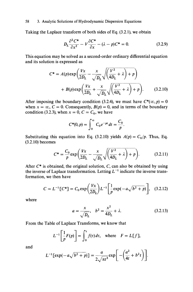
Taking the Laplace transform of both sides of Eq. (3.2.1), we obtain
02C*
oC*
DL ox2 - V ox - (A. - p)C* = o.
(3.2.9)
This equation may be solved as a second-order ordinary differential equation
and its solution is expressed as
(
Vx
x
+ B(p)exp 2D + In
L
yDL
(3.2.10)
After imposing the boundary condition (3.2.4), we must have C*( 00, p) = 0
when x = 00, C = O. Consequently, B(p) = 0, and in terms of the boundary
condition (3.2.3), when x = 0, C = Co, we have
C*(O,p) =
Coe-ptdt =~.
J
oo
C
o
P
Substituting this equation into Eq. (3.2.10) yields A(p) = Co/po Thus, Eq.
(3.2.10) becomes
* Co ( Vx
x J( V 2 ) )
C = pex p 2D L -.,JD;. 4D L + A. + P .
(3.2.11)
After C* is obtained, the original solution, C, can also be obtained by using
the inverse of Laplace transformation. Letting L -1 indicate the inverse transformation, we then have
where
X
x 2
a = - -
b 2 = -
+ A..
.,JD;.'
4DL
(3.2.13)
From the Table of Laplace Transforms, we know that
and
3. Analytic Solutions of Hydrodynamic Dispersion Equations
Taking the Laplace transform of both sides of Eq. (3.2.1), we obtain
02C*
oC*
DL ox2 - V ox - (A. - p)C* = o.
(3.2.9)
This equation may be solved as a second-order ordinary differential equation
and its solution is expressed as
(
Vx
x
+ B(p)exp 2D + In
L
yDL
(3.2.10)
After imposing the boundary condition (3.2.4), we must have C*( 00, p) = 0
when x = 00, C = O. Consequently, B(p) = 0, and in terms of the boundary
condition (3.2.3), when x = 0, C = Co, we have
C*(O,p) =
Coe-ptdt =~.
J
oo
C
o
P
Substituting this equation into Eq. (3.2.10) yields A(p) = Co/po Thus, Eq.
(3.2.10) becomes
* Co ( Vx
x J( V 2 ) )
C = pex p 2D L -.,JD;. 4D L + A. + P .
(3.2.11)
After C* is obtained, the original solution, C, can also be obtained by using
the inverse of Laplace transformation. Letting L -1 indicate the inverse transformation, we then have
where
X
x 2
a = - -
b 2 = -
+ A..
.,JD;.'
4DL
(3.2.13)
From the Table of Laplace Transforms, we know that
and