28
2. Hydrodynamic Dispersion in Porous Media
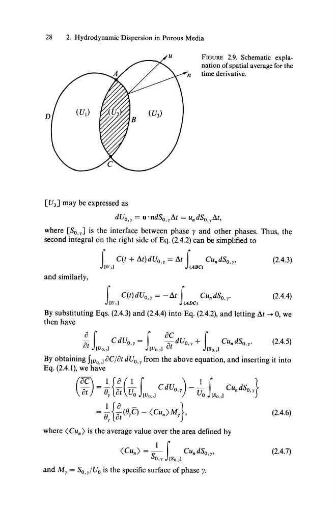
FIGURE 2.9. Schematic explanation of spatial average for the
time derivative.
[U 3 ] may be expressed as
dUo.y = u·ndSo.yAt = undSo.yAt,
where [SO,y] is the interface between phase y and other phases. Thus, the
second integral on the right side of Eq. (2.4.2) can be simplified to
r C(t + At)dUo,y = At r CundSO,y,
J [U 3 1
J (ABC)
(2.4.3)
and similarly,
r C(t)dUo,y = -At r CundSO,y'
(2.4.4)
J [U tl
J (ADC)
By substituting Eqs. (2.4.3) and (2.4.4) into Eq, (2.4.2), and letting At -+ 0, we
then have
:t r C dUo,y = r aa~ dUo,y + r CUn dSo,Y'
J [Uo,,1
J [Uo,,1
J [So,,1
(2.4.5)
By obtaining f[Uo,,1 aC/at dUo, y from the above equation, and inserting it into
Eq. (2.4.1), we have
( ac) 1 {a (1 i ) 1 i }
~ = - - ~
C dUo
- ~
Cu dSo
at
Oy at Uo [Uo,,1
,y
Uo [So,,1
n
,y
1 {a -
}
= ~ at (OyC) - (Cun>My ,
where is the average value over the area defined by
= f- r CundSO,y,
O,y J [So,,1
and My = SojU o is the specific surface of phase y.
(2.4.6)
(2.4.7)