

2.4. Hydrodynamic Dispersion Equations
27
This equation is ealled the convection-difJusion equation of the solute. It is a
seeond-order parabolie partial differential equation. With eertain initial and
boundary eonditions, a unique solution, the eoneentration distribution C,
ean be obtained.
Equation (2.3.10) is derived for a continuous fluid system. If the solute
transport problem is diseussed at the microseopie level, boundary eonditions have to be given along the solid matrices of the porous medium. As
mentioned above, however, these boundary eonditions are impossible to
define due to the eomplexity of microseopic eonstruetures of porous media.
We have to study the problem maeroseopically by means of the spatial
average method.
2.4 Hydrodynamic Dispersion Equations
2.4.1 The Average 01 Time Derivatives
In order to obtain the spatial average for Eq. (2.3.9), the following integration
must be ealculated:
( ac) = _1_ r ac dUo
at
UO,y JIU o .y] at
,y'
(2.4.1)
where [UO,y] is the volume oeeupied by phase y (solution) in the REV [Uo]. If
{}y is the volumetrie fraction ofphase y, then we have UO,y = {}yU o . Consider
a generalized ease whieh is applieable for both unsaturated zones and deformable solid matrices, that is, [UO,y] or {}y is time dependent. Write [UO,y]
at times t and t + At respeetively as follows:
and
[UO,y]/H, = [U2 ] + [U3 ].
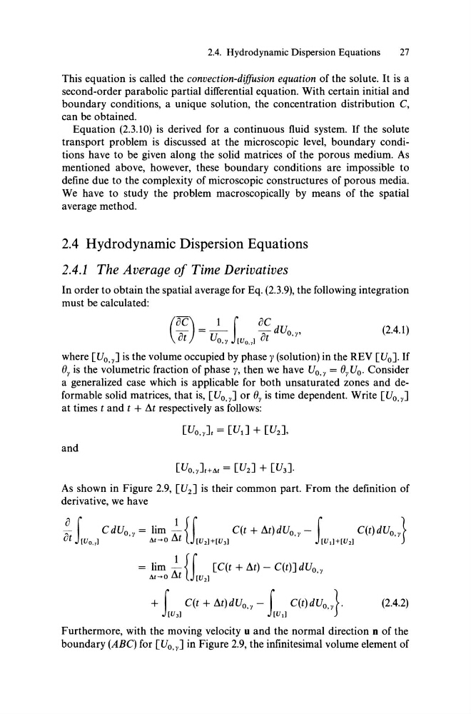
As shown in Figure 2.9, [U 2 ] is their eommon part. From the definition of
derivative, we have
a a r CdUo,y = lim : {r C(t + At)dUo,y - r C(t)dUO,y}
t JIUo. y]
4/ .... 0 ut J[U2]+IU3]
J[Utl+IU2]
= lim : {r [C(t + At) - C(t)] dUo,y
4/ .... 0 ut J IU 2 ]
+ r C(t + At)dUo,y - r C(t)dUO,y}.
JIU3]
JIUtl
(2.4.2)
Furthermore, with the moving velocity u and the normal direetion n of the
boundary (ABC) for [Uo,J in Figure 2.9, the infinitesimal volume element of
27
This equation is ealled the convection-difJusion equation of the solute. It is a
seeond-order parabolie partial differential equation. With eertain initial and
boundary eonditions, a unique solution, the eoneentration distribution C,
ean be obtained.
Equation (2.3.10) is derived for a continuous fluid system. If the solute
transport problem is diseussed at the microseopie level, boundary eonditions have to be given along the solid matrices of the porous medium. As
mentioned above, however, these boundary eonditions are impossible to
define due to the eomplexity of microseopic eonstruetures of porous media.
We have to study the problem maeroseopically by means of the spatial
average method.
2.4 Hydrodynamic Dispersion Equations
2.4.1 The Average 01 Time Derivatives
In order to obtain the spatial average for Eq. (2.3.9), the following integration
must be ealculated:
( ac) = _1_ r ac dUo
at
UO,y JIU o .y] at
,y'
(2.4.1)
where [UO,y] is the volume oeeupied by phase y (solution) in the REV [Uo]. If
{}y is the volumetrie fraction ofphase y, then we have UO,y = {}yU o . Consider
a generalized ease whieh is applieable for both unsaturated zones and deformable solid matrices, that is, [UO,y] or {}y is time dependent. Write [UO,y]
at times t and t + At respeetively as follows:
and
[UO,y]/H, = [U2 ] + [U3 ].
As shown in Figure 2.9, [U 2 ] is their eommon part. From the definition of
derivative, we have
a a r CdUo,y = lim : {r C(t + At)dUo,y - r C(t)dUO,y}
t JIUo. y]
4/ .... 0 ut J[U2]+IU3]
J[Utl+IU2]
= lim : {r [C(t + At) - C(t)] dUo,y
4/ .... 0 ut J IU 2 ]
+ r C(t + At)dUo,y - r C(t)dUO,y}.
JIU3]
JIUtl
(2.4.2)
Furthermore, with the moving velocity u and the normal direetion n of the
boundary (ABC) for [Uo,J in Figure 2.9, the infinitesimal volume element of