

8.3. Groundwater Quality Management Models
283
T ABLE 8.2. The optimal management decision.
Optimal injection rates for each ditch (kgjd)
Ditch
First interval
No.
(0-200 d)
I
ql = 13.3
11
q4 = 12.1
III
q7 = 13.2
FIGURE 8.10. The curves of concentration changes in water
source ditches under the optimal
decision.
Second interval
Third interval
(200-400 d)
(400-600d)
q2 = 10.7
q3 = 13.0
qs = 11.2
q6 = 5.2
qs = 10.5
q9 = 5.9
C(mg/L)
ditch of water source A
o~--~----~--~----~----~~-ditch of water
source C
O~--~500~--~lOOO~--'1~50~O--~2~OOO~~2~5~OO'-t~W~)
where Cj(O, ... , 0, llqi' 0, ... ,0) ean be obtained by solving the simulation
problem in Eq. (8.3.16) subjeet to the eonditions of Eq. (8.3.17) and aU the
corresponding source and sink terms are assigned to be zero, exeept qi' Thus,
all the elements of matrix [R] ean be determined by only solving the simulation problem I times. The last step is to solve the linear pro gram (8.3.22). The
solution for the problem is listed in Table 8.2.
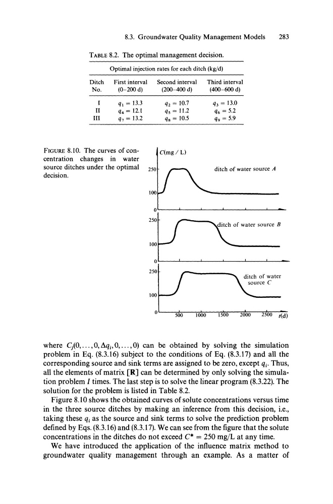
Figure 8.10 shows the obtained eurves of solute eoneentrations versus time
in the three souree ditches by making an inferenee from this decision, i.e.,
taking these qi as the souree and sink terms to solve the predietion problem
defined by Eqs. (8.3.16) and (8.3.17). We ean see from the figure that the solute
coneentrations in the ditehes do not exceed C* = 250 mg/L at any time.
We have introdueed the applieation of the influence matrix method to
groundwater quality management through an example. As a matter of
283
T ABLE 8.2. The optimal management decision.
Optimal injection rates for each ditch (kgjd)
Ditch
First interval
No.
(0-200 d)
I
ql = 13.3
11
q4 = 12.1
III
q7 = 13.2
FIGURE 8.10. The curves of concentration changes in water
source ditches under the optimal
decision.
Second interval
Third interval
(200-400 d)
(400-600d)
q2 = 10.7
q3 = 13.0
qs = 11.2
q6 = 5.2
qs = 10.5
q9 = 5.9
C(mg/L)
ditch of water source A
o~--~----~--~----~----~~-ditch of water
source C
O~--~500~--~lOOO~--'1~50~O--~2~OOO~~2~5~OO'-t~W~)
where Cj(O, ... , 0, llqi' 0, ... ,0) ean be obtained by solving the simulation
problem in Eq. (8.3.16) subjeet to the eonditions of Eq. (8.3.17) and aU the
corresponding source and sink terms are assigned to be zero, exeept qi' Thus,
all the elements of matrix [R] ean be determined by only solving the simulation problem I times. The last step is to solve the linear pro gram (8.3.22). The
solution for the problem is listed in Table 8.2.
Figure 8.10 shows the obtained eurves of solute eoneentrations versus time
in the three souree ditches by making an inferenee from this decision, i.e.,
taking these qi as the souree and sink terms to solve the predietion problem
defined by Eqs. (8.3.16) and (8.3.17). We ean see from the figure that the solute
coneentrations in the ditehes do not exceed C* = 250 mg/L at any time.
We have introdueed the applieation of the influence matrix method to
groundwater quality management through an example. As a matter of