

8.3. Groundwater Quality Management Models
279
(b 1 ,b 2 , ... ,b m f; and
OSI OSI
OSI
oPI oP2
oPm
OS2 OS2
OS2
[A] = oPI oP 2
oP m
(8.3.10)
oSm oSm
oSm
oP I oP 2
oP m
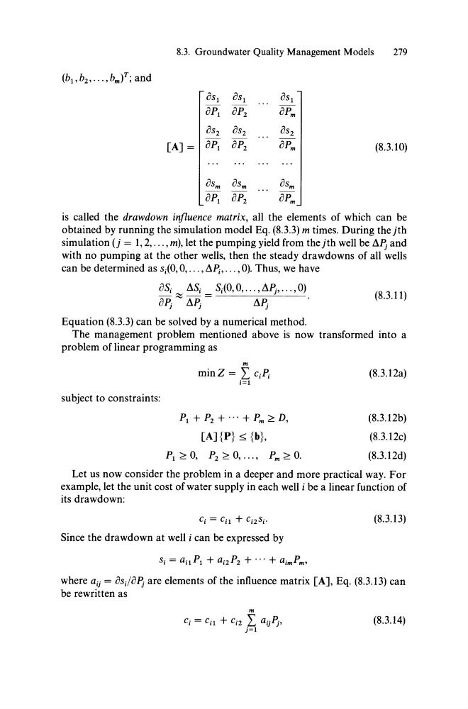
is called the drawdown inj7uence matrix, all the elements of which can be
obtained by running the simulation model Eq. (8.3.3) m times. During the jth
simulation (j = 1,2, ... , m), let the pumping yield from the jth weIl be ~~ and
with no pumping at the other weIls, then the steady drawdowns of all wells
can be determined as Si(O, 0, ... , ~Pi' ... ' 0). Thus, we have
OSi
~Si
Si(O, 0, ... , ~~, ... , 0)
o~ ~ ~~ =
~~
(8.3.11)
Equation (8.3.3) can be solved by a numerical method.
The management problem mentioned above is now transformed into a
problem of linear programming as
subject to constraints:
m
min Z = L: CiPi
i;1
PI + P 2 + ... + Pm ~ D,
[A] {P} ~ {b},
(8.3.12a)
(8.3.12b)
(8.3.12c)
(8.3.12d)
Let us now consider the problem in a deeper and more practical way. For
example, let the unit cost of water supply in each weIl i be a linear function of
its drawdown:
(8.3.13)
Since the drawdown at weIl i can be expressed by
where aij = osjo~ are elements of the influence matrix [A], Eq. (8.3.13) can
be rewritten as
m
Ci = Cil + Ci2 L aij~'
j;1
(8.3.14)
279
(b 1 ,b 2 , ... ,b m f; and
OSI OSI
OSI
oPI oP2
oPm
OS2 OS2
OS2
[A] = oPI oP 2
oP m
(8.3.10)
oSm oSm
oSm
oP I oP 2
oP m
is called the drawdown inj7uence matrix, all the elements of which can be
obtained by running the simulation model Eq. (8.3.3) m times. During the jth
simulation (j = 1,2, ... , m), let the pumping yield from the jth weIl be ~~ and
with no pumping at the other weIls, then the steady drawdowns of all wells
can be determined as Si(O, 0, ... , ~Pi' ... ' 0). Thus, we have
OSi
~Si
Si(O, 0, ... , ~~, ... , 0)
o~ ~ ~~ =
~~
(8.3.11)
Equation (8.3.3) can be solved by a numerical method.
The management problem mentioned above is now transformed into a
problem of linear programming as
subject to constraints:
m
min Z = L: CiPi
i;1
PI + P 2 + ... + Pm ~ D,
[A] {P} ~ {b},
(8.3.12a)
(8.3.12b)
(8.3.12c)
(8.3.12d)
Let us now consider the problem in a deeper and more practical way. For
example, let the unit cost of water supply in each weIl i be a linear function of
its drawdown:
(8.3.13)
Since the drawdown at weIl i can be expressed by
where aij = osjo~ are elements of the influence matrix [A], Eq. (8.3.13) can
be rewritten as
m
Ci = Cil + Ci2 L aij~'
j;1
(8.3.14)